Query Processing
Read in Elmasri & Navathe (EN)
- EN6 Chapter 19 / EN7 Chapter 18: Algorithms for Query Processing
- EN6 Chapter 20 / EN7 Chapter 19: Query Optimization
How should a database organize the execution of a query?
How can we identify slow queries?
How can we make them run faster?
In this section we will assume that multiple records are
stored per disk block, and that the goal of query
optimization is to minimize the number of block reads.
Ideally this material would be read after the files_and_indexes.html
material, but this is not essential. A B-Tree index is a very "fat" tree
that is ordered by the key value in question. The ordering means that a
B-Tree can be used either for single-value queries, e.ssn
= '111223333', or range queries: e.ssn
between '111223333' and '111229999'.
To begin, note it is relatively easy to sort
records. Typically we will use merge-sort, where we subdivide into blocks
small enough to fit into memory. We sort those with, say, quicksort. We then
make passes until each pair of consecutive blocks is merged.
Select
Some examples
- select * from employee e where e.ssn = '123456789'
- select * from department where dnumber >=5
- select * from employee where dno = 5
- select * from employee where dno = 5 and salary > 30000 and sex =
'F'
- select * from works_on where essn='123456789' and pno=10
Methods of implementation:
Linear search: we read each disk
block once. This corresponds to a search
for e in employee ....
Binary search: this is an option if
the selection condition is an equality test on a key attribute, and the file
is ordered by that attribute.
Primary index: same requirement as
above, plus we need an index
Hash search: equality comparison on
any attribute for which we have a hash index (need not be a key attribute)
Primary index and ordered comparison:
use the index to find all departments with dnumber > 5
Clustered index (includes hash
indexes)
B-tree index
If we are searching for "dno=5 AND salary=4000" we can use an index for
either attribute, or a composite index if one exists.
In general, we would like to start with the condition that leads to the fewest results, and then continue with
the remaining conditions.
For OR conditions, we just have to search for each.
For the examples above, here are some notes on which select
implementation is likely to be most efficient.
- For this query, an index on employee.ssn is likely to be fastest. Any
index will do.
- For this query, the range comparison (dnumber >=
5) means that unless we have an "ordered" index (that is, a B-tree or a
"primary index") we might find linear search hard to beat. Note that
this is a search by key attribute.
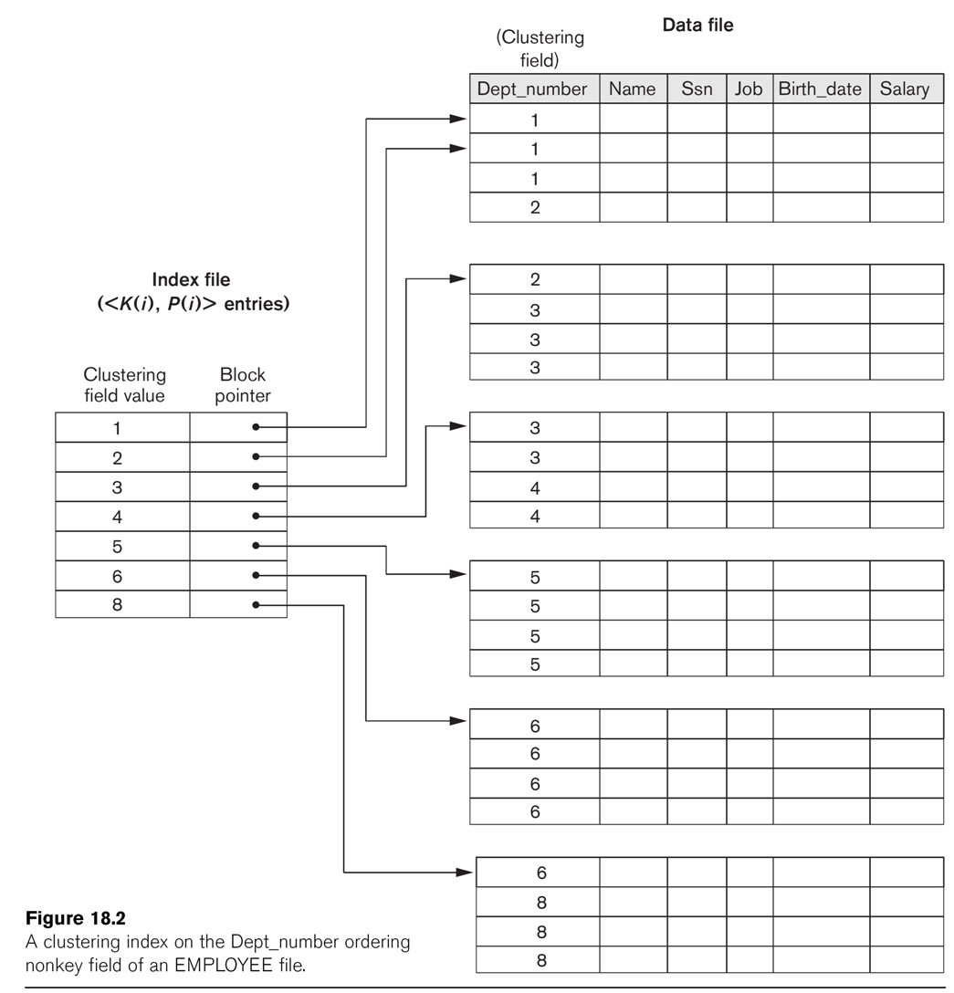
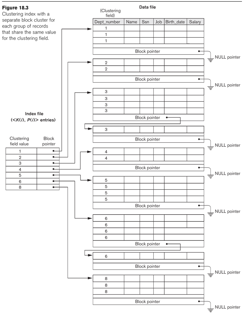
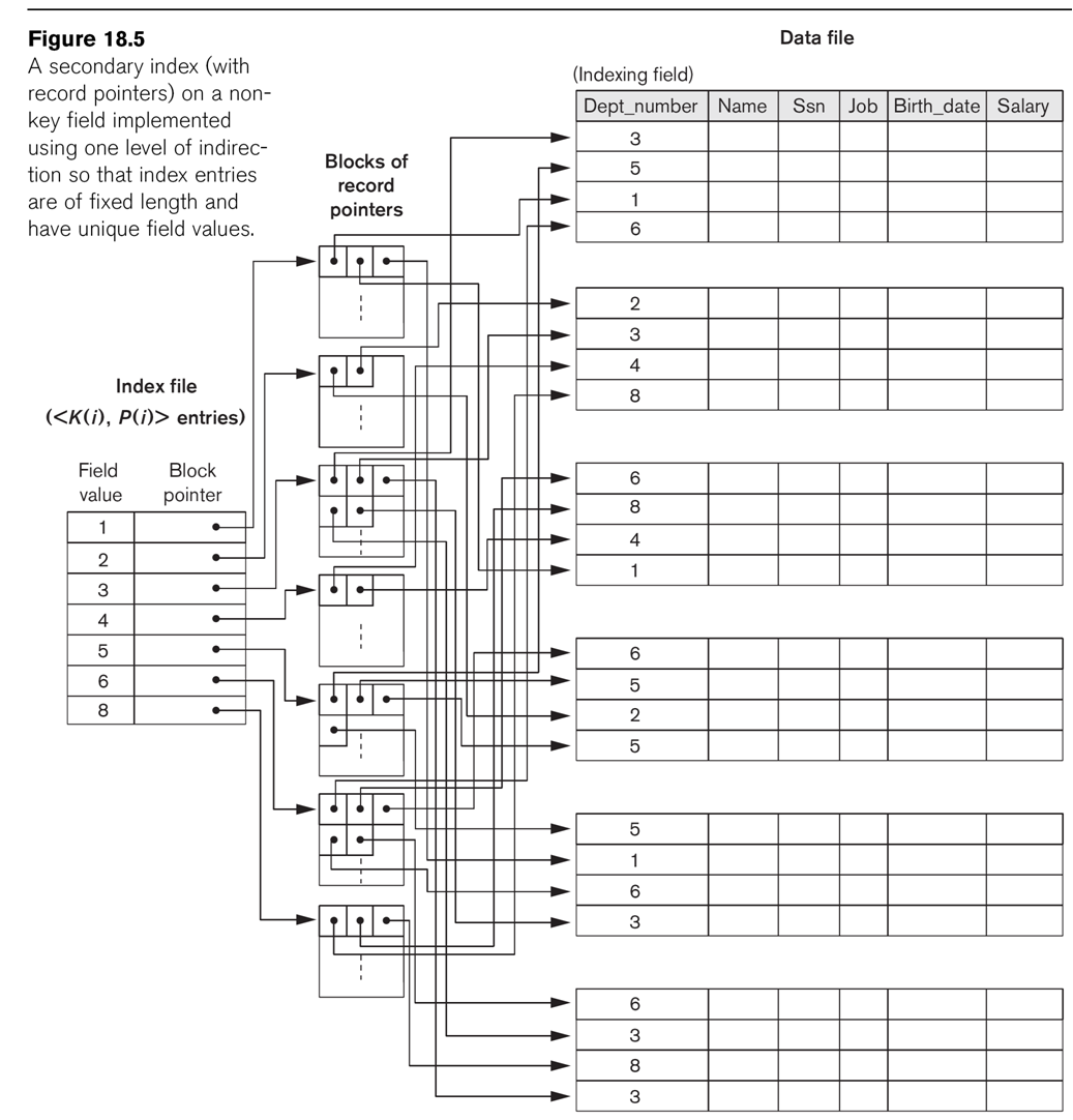
- For this query, an index on dno would be a clustering index as in figs
18.2, 18.3
and 18.5. This index could be used,
and if the employee file were ordered by dno then the minimum number of
blocks would need to be retrieved. But this is unlikely; and that in
turn means that using the index might still involve retrieving nearly
ever block of the employee file (for example, if almost every block
contained at least one member of department 5). Linear search in such a
case would be hard to beat.
- In this case we have three selection criteria. We are best off
applying the most selective criterion first. Unless we know
something about the distribution of salaries, we can assume that
"salary>30000" is about 50% likely to be true; the same might be true
for "sex = 'F'". We are best off starting with dno=5, and then searching
only those records for the ones that also satisfy the other two
criteria.
- Note that the primary key to works_on is the pair (essn,pno). If we
have a primary-key index, we can simply look this up. But if we keep the
file ordered by essn, and with an index on essn, then we can also use
that to find the answer; most employees work on only a small number of
projects so works_on.lookup(essn) will be small.
Scans
Here are three types of scans:
1. Heap scan (or sequential scan): we go through the
table a block at a time
2. Index scan: we go through the table via accessing
the index, a record at a time. Normally, going through record by record is
inefficient, but we may not actually need to access anything besides the
index. Often, we can eliminate many records based only on information
available in the index.
In some cases the scan requires only the information found in
the index; we don't have to retrieve data blocks from the table at all. In
this case, the scan is an index-only scan.
3. Bitmap heap scan: we go through the index, but then
sort the record addresses by block, and then go through the records
block-by-block. This resembles a heap scan, but we can do the following:
- eliminate some records in the initial pass, based on information
available in the index
- use two different indexes. Each generates a list of blocks. We then
intersect the lists, to get possible locations of records satisfying a
condition on each index (think "salary < 4000 and dno=4"). As the
list of block addresses is usually maintained in a bitmap, intersecting
the lists simply involves taking the bitwise AND.
Joins
Mostly we focus on equijoins:
- select * from employee e join department d on e.dno = d.dnumber
- select * from department d join employee e on d.mgr_ssn = e.ssn
In each case we are joining a key in one table (underlined) to a foreign key
in another. However, it is likely that the employee table is much larger
than the department table. In the first example, the number of records in
the join will be (about) the size of the employee table (that is, large); in
the second example the number of records in the join will be (about) the
size of the department table, much smaller. Thus, while both are joins of
the employee and department tables, the joins are in fact quite different.
We will consider four methods of implementation.
Numeric examples for the four methods (EN6 p 690-693): Suppose we have 6,000
employee records in 2,000 blocks, and 50 departments in 10 blocks. We have
indexes on both tables. The employee.ssn index takes 4 accesses, and the
dept.dnumber index takes 2.
1. Nested-loop join: this is where
we think of a for-loop:
for (e in employee) {
for (d in department) {
if (e.dno = d.dnumber)
print(e,d);
}
}
The time needed here is NM, where N is the size of employee and M is the
size of department; loosely speaking, we might say this is quadratic.
If we go through the employee table record by record, that amounts to 2,000
block accesses. For each employee record
the loop above would go through all 10 blocks of departments; that's 6,000 ×
10 = 60,000 blocks. Doing it the other way, we go through 50 department
records, and, for each department record, we search 2,000 blocks of
employees for 50×2,000 = 100,000 block accesses. In other words, the
complexity is not symmetric!
However, note that we can also do this join block-by-block
on both files (sometimes called the block-nested-loop
approach):
- read a block of employees
- read a block of departments
- search both for any join instances
- go on to the next block of departments
Done this way, the number of block accesses is 2,000 × 10 = 20,000 blocks,
or, in general, NM, where N and M are now the sizes of the respective tables
in blocks.
Realistically, doing operations block-by-block instead of
record-by-record is very important!
Performance improves rapidly if we can keep the smaller table entirely in
memory: we then need only 2,010 block accesses! (The EN6 analysis makes some
additional assumptions about having spare buffer blocks to work with.)
All joins in MySQL (5.7) are considered to be nested-loop joins, although
MySQL considers index joins to be a special case of nested-loop joins. MySQL
does not implement hash or sort-merge joins. Block-nested-loop
joins are used where possible.
2. Index join: if we have an index
on one of the attributes, we can use it to find the joined records. Here is
an example using the index on d.dnumber; it might be used to implement the
query select * from department d join
employee e on d.dnumber = e.dno.
for (e in employee) {
d = lookup(department, e.dno);
if (d != null) print(e,d);
}
Note that any index will do, but that this may
involve retrieving several disk blocks for each e and will almost certainly
involve retrieving at least one disk block (from department) for every e in
employee. It may or may not be better than Method 1.
Consider the first query above. Suppose we have a primary index on
department.dno that allows us to retrieve a given department in 2 accesses.
Naively, we go through 6,000 employees and retrieve the department of each;
that's 6,000×2 = 12,000 block accesses. There is no obvious way to take
advantage of the grouping of employees into blocks (why?).
Now consider the second query, and suppose we can find a given employee in 4
accesses. Then we go through 50 × 4 = 200 block accesses (for every
department d, we look up d.mgr_ssn in table employee). Of course, as we
noted at the beginning, the final result of the second query is a much
smaller table.
3. Sort-merge join: we sort both
files on the attribute in question, and then do a join-merge. This takes a
single linear pass, of size the number of blocks in the two files put
together file. This is most efficient if the files are already
sorted, but note that it's still faster than 1 (and possibly faster than 2)
if we have to sort the files. Assume both tables are sorted by their primary
key, and assume we can sort in with N log(N) block accesses, where N is the
number of blocks in the file. Then query 1 requires us to sort table
employee in time 2,000×11 = 22,000; the actual merge time is much smaller.
Query 2 requires us to sort table department in time 10×4 = 40; the merge
then takes ~2,000 blocks for the employee table.
4. Hash (or partition-hash) join:
Let the relations (record sets) be R and S. We partition R into disjoint
sets Ri = {r ∈ R | hash(r) = i}, and S into Si = {s∈S
| hash(s) = i}. Now we note that the join R ⋈ S is simply the disjoint union
of the Ri ⋈ Si. In most cases, either Ri or
Si will be small enough to fit in memory.
If R is small enough that we can keep all the Ri in memory, the
process is even simpler: we create the Ri, and then make a single
scan through S. For each record of s, we use the hash function to figure out
which Ri we need to search, and then search that Ri
for a match.
A good hash function helps; we want the buckets to be relatively uniform. We
won't get uniform distribution, but we should
hope for Poisson distribution. With N things in K buckets, we expect an
average of a=N/K per bucket. The probability of i things is aie-a/i!
and the expected number of i-sized buckets is about N*aie-a/i!.
An important feature of hash joins is that an index is not necessary.
The join selection factor is the
fraction of records that will participate in the join. In query 2 above,
select * from department d, employee e where d.mgr_ssn =
e.ssn
all departments will be involved in the join, but almost
no employees. So we'd rather go through the departments, looking up
managing employees, rather than the other way around.
In the most common case of joins, the join field is a foreign key in one
file and a primary key in the other. Suppose we keep all files sorted by
their primary key. Then for any join of this type, we can traverse the
primary-key file block by block; for each primary-key value we need to do a
lookup of the FK attribute in the other file. This would be method 2 above;
note that we're making no use of the primary index.
Query optimization
As with compilers, the word "optimization" is used loosely. However, SQL
statements can usually be implemented a number of ways.
A major rule is to apply select/project before joins, and in general do
operations first that have greatest potential for reducing the size of the
number of records. But if projection makes an index unavailable, and the
index would speed up the join, do it later (that is, use the index).
Query tree: See fig 19.4.
Select lname from employee e, works_on w, project p
where e.ssn = w.essn and w.pno = p.pnumber and p.pname = 'Aquarius';
See fig 19.5, but note that doing
cross-products was never on the
agenda. However, it still does help to do the second join first.
Some heuristic rules:
- Move the more-restrictive SELECT operations down towards the leaf
nodes; that will reduce number of records. (But note that once you do a
SELECT, you lose the index).
- Same with PROJECT; try to do joins last
- Do the joins in the right order, using the join selection factor
estimate
- Do the smaller joins first (or, more generally, do the joins that will
result in an absolutely smaller set of records, whether this is because
the relations were small to start with or because one condition was
highly selective).
For information on how MySQL organizes queries, including the explain
command, see admin1.html#explain.
Selecting Indexes
Much of this information comes from www.slideshare.net/myxplain/mysql-indexing-best-practices-for-mysql
and www.slideshare.net/billkarwin/how-to-design-indexes-really.
The first step is identifying which queries are underperforming. If a
query is slow, but you don't run it often, it doesn't matter. The MySQL
slow-query log (/var/log/mysql/mysql-slow.log) can be useful here.
If a query is not running fast enough, options available include
- adding options to force the query to be run a certain way
- restructuring the query, eg from a nested query to a join
- adding suitable indexes
The straight_join option (above) is often useful for
the first category, as can be the addition of a WITH INDEX index_name
option. Most query-optimizing efforts, however, are in the last category:
adding indexes.
Be aware that indexes add write costs for all updates; don't create more
than you need.
A B-Tree index can also be used to look up any prefix of the key. The
prefix might be a single attribute A in an index on trow attributes (A,B),
or else a string prefix: e.ssn LIKE '55566%'.
B-tree indexes can also be used for range queries: key < 100, key
BETWEEN 50 AND 80, for example.
Join comparisons do best when the fields being compared are both strings
and are both the same length. Joining on ssn where one table declares ssn
to be an Integer and the other a CHAR(9) is not likely to work well.
A non-key index has high selectivity if each index
value corresponds to only a few records. An index on lname might qualify.
The standard example of a low-selectivity index is one on sex.
Many MySQL indexes on a non-key field A are really dual-attribute indexes
on (A,PK) where PK is the primary key.
In a multi-attribute index, MySQL can use attributes up until the first
one not involved in an equality comparison (that is, not used or involved
in an inequality). If the index is on attributes (A,B,C), then
the index can be used to answer:
A>10
A=10 and B between 30 and 50
A=12 and B=40 and C<> 200
The telephone book is an index on (lname, fname). It can find people with
lname='dordal' quickly, but is not very useful in finding people with
fname='peter'.
Sometimes a query can be answered by using ONLY the index. In that case,
the index is said to be a covering index for that query.
For example, if we have an index for EMPLOYEE on (dno,ssn), then we can
answer the following query using the index alone:
select e.ssn from employee e where e.dno = 5
The (dno,ssn) index is a covering index for this query.
For the phone book, an index on (lname, fname, phone) would be a covering
index for phone-number lookups, but not, say, for address lookups.
For the works_on table, an index on (essn,pno,hours) ((essn,pno) is the
primary key) is a covering index for the whole table.
If the query is
select e.lname from employee e where e.salary
= 30000 and e.dno = 5;
then while the ideal index is a common index on either (salary,dno) or
(dno,salary), two separate indexes on (salary) alone and on (dno) alone
are almost as useful, as we can look up the employees with salary = 30000
and the employees in dno 5 and then intersect the two sets. The strategy
here is sometimes called "index merge".
Sometimes, if the key is a long string (eg varchar(30)), we build the
index on just a prefix of the string (maybe the first 10 characters). The
prefix length should be big enough that it is "selective": there should be
few records corresponding to each prefix. It should also be short enough
to be fast. If a publisher database has an index for book_title, of max
length 100 characters, what is a good prefix length? 10 chars may be too
short: "An Introdu" matches a lot of books. How about 20 characters? "An
Introduction to C" is only marginally more specific.