Comp 305/488: Database Administration, LT 410, 4:15 Tuesdays
Miscellaneous database administration notes
Mostly relating to INDEXES and QUERY
OPTIMIZATION (including EXPLAIN)
(And some on Oracle)
A Big Dataset
I downloaded 10,000,000 ⟨username,password⟩ pairs from xato.net/passwords/ten-million-passwords.
This is real password data; users chose their passwords with the expectation
that they would not be seen by others.
All the pairs are in Postgres in the table passwords.password on ulam, and
in MySQL on host sql1. I first modified the data to replace control
characters and non-Ascii Unicode characters with reasonable Ascii
equivalents.
Auxiliary goals:
- legitimize the data by putting it to a non-hacking use
- establish the legitimate use of bittorrent
The size of the Ascii tables files is about 200 Mbyte. The actual MySQL
file with index is about four times that, but only a little over twice
that without the index (perhaps because I allowed varchar(80?)
-rw-rw----
1 mysql mysql 801112064 Feb 17 12:22 password.ibd
-rw-rw---- 1 mysql mysql 478150656 Feb 17 12:11 password_noindex.ibd
For Postgres, the file size without index was 500,998,144 bytes. With
index, the base file didn't change size.
See here for file locations.
Copying the table within MySQL takes about 1.5 minutes. Copying in
Postgres took 164 seconds, or 2.75 minutes.
The password table was defined as follows:
create
table password (
username varchar(80) not null,
password varchar(80) not null,
primary key(username,password)
)
The csv text files can be loaded into the table (as user postgres) using
copy password from 'filename' delimiter E'\t'
csv;
How many entries?
select
count(*) from password;
Whose password is the same as their username?
select
count(*) from password p where p.username = p.password;
219058
1 row in set (7.94 sec) (MySQL)
This query requires one pass through the data. The time here is typical of
such a pass. For Postgres, the time was just over 10 seconds. The command
\timing enables query timing in Postgres.
Next let's compare the results of two similar queries:
select
* from password where username = A
select * from password where
password = B
Here are a few (A,B) pairs to try, where in each case both the username and
password are unique.
badmole,
150super
corydeut, uxoodo
eurotags, Lambrech
hpgator, ncgator
kiraartmank, sundayfunday
megabit_tat, Rafit03
pasdebois123, gingerpasdecalai
sargis88ov, sarkisov
telo4ela, qazZZ1234
zypipofylyk, KArIHaFacEH
Times to look up a username are reported by MySQL as 0.00, and by
Postgres as in the range 0.5-20 ms. Times to look up a password are ~7.6
seconds in MySQL and ~10 seconds in Postgres. Why the difference?
The original password table has a primary key, and therefore, automatically,
an index on that key. An index greatly improves the speed
of a lookup given a key value.
Here, though, the key values have two attributes:
⟨username,password⟩. In this case, MySQL indexes support fast prefix
lookup: given just a username, we can quickly find all the
matching ⟨username,password⟩ pairs. This works just like using a phone book,
which is an index on ⟨lastname,firstname⟩ pairs, to look someone up using
only the last name.
In MySQL I also created a copy of the table, password_noindex, with no
key and therefore no index at all:
create
table password_noindex (
username
varchar(80) not null,
password
varchar(80) not null
)
How do the lookup times compare with this table?
We can add a second index to the original table, on just the password.
create
index pwindex on ipassword(password); -- took
show index from ipassword;
-- Mysql; in
postgres use \d ipassword
drop index pwindex on
ipassword;
Index creation takes about 1 minute 50 seconds in MySQL, and 3 min 40
seconds in Postgres. I did this to a copy of table password, named password2
in MySQL and ipassword in Postgres, so we could have both forms of the table
simultaneously.
What effect does the presence of pwindex
have on the lookups?
Now let's count usernames and passwords matching a string condition:
select
count(username) from password where username like 'david%';
select count(username) from
password where username like '%david%';
select
          count(*) from password where password like 'david%';
select count(*) from password where
password like '%david%';
The first search here is still a prefix search using the primary-key index;
the other searches are not. Why?
MySQL automatically uses an index on username for the first (username like
'david%') query. Postgres does not, by default, and so this query takes the
same ~10 seconds as the others, and is based on sequential search.
But we can configure the index so that it does use text
prefixes, with the varchar_pattern_ops
or text_pattern_ops options.
I added an index "username_prefix" using the text_pattern_ops option to
table password, speeding up this username
like 'david%' query from 10 seconds to 164 ms. Here's the create
table code:
create
table ipassword (
username
varchar(80) not null,
password
varchar(80) not null,
primary
key(username,password)
);
create
index password_index on ipassword (password);
create
index username_prefix on ipassword (username, password
varchar_pattern_ops);
This last index took 61 seconds to create. Back to the index-as-phonebook
analogy, if you know lastname='Smith', you turn to the Smith pages and start
searching for firstname. The same works, though, if you know lastname starts
with 'Smi'. The reason Postgres does not enable varchar_pattern_ops as the
default, by the way, is that it requires using the locale character
collation order, and this is often not set.
How fast are these queries using table password versus table
password2/ipassword?
Counting distinct entries
Next we count the number of distinct usernames and unique passwords, without
the secondary index:
select
count(distinct username) from password;
8106113
1 row in set (21.57 sec) -- Postgres took 140 sec
select
count(distinct password) from password;
5054219
1 row in set (26.30
sec) -- Postgres took 186 sec
Both these queries require a sort to eliminate duplicates. There is not much
penalty, however, for using the non-indexed value. An index doesn't help
with sorting.
Here we count usernames occuring >= 100 times:
select
username, count(password) from password group by username having
count(password) >=100;
1205 rows in set (0.00 sec)
What about a similar count for passwords?
select
password, count(username) from password group by password having
count(username) >= 100;
5062 rows in set (4 min 2.23 sec)
If we change the comparison to >=1000, we get 188 rows in the set (4 min
4.92 sec).
What happens to the time here if we re-create the password index?
Counting items that occur only once
How can we count usernames that occur only a single time? One way is to use
HAVING, along with an inner query. Selecting from an inner
query requires that we give the inner query a table-alias name, TEMP.
select
          count(*) from

        (select username, count(password)
          from password group by username having count(password) = 1) as TEMP;
7465978
MySQL: 18-25 seconds
Postgres: 142 seconds
But the second time we run this we get: 1 row in set (0.00 sec). Why the
speedup? Because MySQL remembers table TEMP (or maybe it remembers the query
itself). Change it to TEMP2 and the time is back up to 18 seconds. I am not
sure how long MySQL remembers TEMP.
Another way to do this query is with NOT EXISTS. This is
slower in MySQL, but faster in Postgres:
select
count(*) from password p where not exists (select * from password p2
where p.username = p2.username and p.password <> p2.password);
7465978
MySQL: 1 min 1.31 sec Postgres: 119 sec
Here is a slightly different formulation, again using a subquery but also
NOT EXISTS:
select
count(*) from (select * from password p where not exists (select * from
password p2 where p.username = p2.username and p.password <>
p2.password)) as T;
7465978
MySQL: 1 min 17.96 sec
To an extent, the slowness is fundamental: for each p, we have to search the
table for records p2 that match.
Finally, we can use a LEFT JOIN. The idea is to join the
password table to itself on the condition that usernames match but passwords
do not, and then look only at records where the join failed. Note the double
join condition for a single join.
select
count(*) from password p left join password p2 on (p.username =
p2.username and p.password <> p2.password) where p2.username is
null;
7465978
MySQL: 48.81 sec
Postgres: 129 sec
With the index on password2.password, the HAVING query takes about the same
amount of time. The NOT EXISTS query takes much longer, 10 min 37.57 sec!
The LEFT JOIN query also takes much longer: 9 min 23 sec. What happened? I'm
still working on this, but it appears that MySQL was misled by the
second index, and attempted to use it for individual lookups when that
strategy was ultimately slower.
Now let's try these to count unique passwords rather than
usernames. Does the lack of an index slow us down?
select
count(*) from
(select password, count(username)
from password group by password having count(username) = 1) as TEMP;
select
count(*) from password p where not exists (select * from password p2
where p.password = p2.password and p.username <> p2.username);
select
count(*) from password p left join password p2 on
(p.password = p2.password and p.username <> p2.username) where
p2.password is null;
If we run the first query here on table password, it takes MySQL 6 min 59
sec, returning a count of 4300984. If we run it on table password2, with
index pwindex, it takes 30 sec. This is a big speedup with the index!
Here's a more direct variant on counting usernames using the same password:
select
password, count(username) from password group by password having
count(username) >= 2000;
MySQL and Postgres each took between 4 and 4.5 minutes.
One caveat: the tables are big enough that accessing a
second table has a material effect on the buffer pool, which in turn can
have a big effect on timing. But, over multiple runs, I seldom saw
variations in excess of 10%.
Here are some older Postgres timing values from my old (iron-disk) laptop
select
* from password where password = 'uxoodo';
corydeut | uxoodo
Time: 12910.541 ms
Not so impressive. Again:
select
* from password where password = 'Lambrech';
4104.560 ms
Better! Again:
select
* from password where password = 'ncgator';
Time: 2629.510 ms
How about uxoodo again?
Time: 2758.630 ms
The first time took ~13 seconds. Then 4, and then (pretty stably, even if
the queries get repeated a while) ~2.7 seconds.
What is going on?
Why is this speeding up? This is probably related
to a rather large disk cache.
Bigger Company
The Company has had a hiring spree. I created data for 300 more
employees, and a total of 20 departments and 40 projects. Each new
employee works on four projects. This data is in my database bigcompany,
available at pld.cs.luc.edu/database/bigcompany.
(Only tables employee, department, project and works_on are provided; you
can use the original versions of the other files, or leave them out.)
The new employee names all came courtesy of listofrandomnames.com
(who would have thought?). The new hires don't have addresses yet, though
I did give them random salaries.
Most of the employee data was created using C# programs that generated
appropriate insert/update statements using random values. The new
employees have ssns from 111220001 to 111220300.
Select
count(*) from employee;
returns 308
select
e.ssn, e.fname, e.lname, e.salary, e.dno from employee e order by
e.lname limit 50;
The limit N SQL clause is
useful at the end of any query to view only some of the data.
A few notes on transferring data from MySQL to Postgres:
(Generally, export and import must be run as "root" or "superuser")
To export: select * from employee into outfile
'/home/pld/bigemployee.csv';
To import into postgres, run the following. To use the copy command, you
have to be the postgres user.
\connect
bigcompany
copy employee
from '/home/pld/305/bigcompany/bigemployee.csv'
delimiter E'\t' csv null '\N';
copy department
from '/home/pld/305/bigcompany/bigdepartment.csv' delimiter E'\t'
csv null '\N';
copy project
from '/home/pld/305/bigcompany/bigproject.csv'
delimiter E'\t' csv null '\N';
copy works_on
from '/home/pld/305/bigcompany/bigworks_on.csv' delimiter
E'\t' csv null '\N';
A performance experiment
Here is table foo:
describe foo;
+-------+--------------+------+-----+---------+-------+
| Field | Type         | Null | Key | Default | Extra |
+-------+--------------+------+-----+---------+-------+
| id    | int(11)      | YES  |     | NULL    |       |
| name  | varchar(100) | YES  |     | NULL    |       |
+-------+--------------+------+-----+---------+-------+
select * from foo;
+------------+-------+
| id         | name  |
+------------+-------+
|          1 | peter |
|          3 | ralph |
| 2147483647 | fred  |
+------------+-------+
I then ran 1000 update queries from the command line, using a shell script,
and measured the time. These measurements were done with MySQL 5.5, in 2013.
time
while [ $n -lt 1000 ]
do
n=$(expr $n + 1)
mysql --password="ZZZ" -D plddb -e "update foo set
id=id+1 where name='peter'"
done
real 0m43.659s
user 0m3.280s
sys 0m2.640s
That's 23 updates per second.
If I do this just with a query:
time
while [ $n -lt 1000 ]
do
n=$(expr $n + 1)
mysql --password="blue" -D plddb -e "select name from
foo where id=3"
done > /dev/null
Then the time is about 9.35 seconds (11.9 seconds if output is not sent to
/dev/null). That's about 1 query every 10 ms.
I really should run the queries from, say, a PHP program. Still, this
illustrates a pretty dramatic difference between reading and writing.
Explain in MySQL
Most SQL implementations provide an explain command to
report how a database organizes a query's execution. This section has
examples from MySQL; the following section has examples from Postgres.
Official documentation for MySQL explain is
at https://dev.mysql.com/doc/refman/5.6/en/explain-output.html.
Here is an example. Suppose the query is the following triple
join:
select e.lname, p.pname, w.hours
from employee e, project p, works_on w
where e.ssn = w.essn and w.pno = p.pnumber
If we run this on the bigcompany data using MySQL 5.7:
explain select e.lname, p.pname, w.hours
        from employee e, project p, works_on w where e.ssn = w.essn and w.pno =
        p.pnumber;
we get a table:
| id |
select_type |
table |
type |
possible_keys |
key |
key_len |
ref |
rows |
Extra |
| 1 |
simple |
e |
ALL |
primary |
NULL |
NULL |
NULL |
308 |
NULL |
| 1 |
simple |
w |
ref |
primary,pno |
primary |
9 |
e.ssn |
1 |
NULL
|
| 1 |
simple |
p |
eq_ref |
primary |
primary |
4 |
w.pno |
1 |
NULL
|
The rows here refer to the individual tables of the join, identified by
their table aliases in the table column. Other columns
are as follows:
- select_type: simple means a simple
join, with no nested subquery.
- type:
- index means the index was scanned in full. This is
slightly faster than scanning the table row-by-row.
- ref means that all matching rows (in a join) were
retrieved. An index is used, but it is not a key index. Above, given a
project record, all matching works_on rows with that project.pnumber
are retrieved using the works_on.pno index.
- eq_ref means that MySQL knew there would be only
one matching row (eg the lookup of w.essn in table employee). This is
only used if there is a suitable key index available. MySQL looks up
the matching row using the index. Above, given a works_on record w,
MySQL looks up w.essn in employee using the index on employee.ssn.
- all: all records were examined
- const: MySQL knows there is a single match
- possible_keys: list of keys that might have been used
- key: the actual key that was used
- key_len: the length of the key, in bytes. The
department.dname key is of type varchar(15); the extra two bytes are
presumably a length field.
- ref: what value was looked up in this table (for
example, p.pnumber was looked up in the works_on table using the pno
index)
- rows:An estimate of the number of rows to be
examined. When looking up w.essn in table employee, the 1 here is exact,
as ssn is the primary key of employee. When looking up p.pnumber in
works_on, the 1 is a gross underestimate. It is not
exactly clear why this is happening; the fact that the type column is ref
rather than eq_ref shows that MySQL knows one
p.pnumber value may lead to multiple works_on matches.
- extra: Additional information as appropriate. The
"using index" here means that each project name is looked up via the
index, rather than simply by traversing the project table row-by-row.
What MySQL did here was to
- First retrieve every employee (the ALL in the type
column), using the employee.ssn (primary-key) index.
- For each e.ssn value (column ref), retrieve matching
works_on records using the works_on.essn index (the PRIMARY index). The
ref in the type column means that this is a
one-to-many lookup (as only one of the two primary-key fields are used).
The 1 in the rows column is
misleading.
- For each record so far, look up the pno (column ref)
in the project table. The eq_ref in the type column
shows that MySQL knows these matches must be unique.
Here is a closely related query:
select e.lname from employee e, works_on w,
project p
where e.ssn = w.essn and w.pno = p.pnumber and p.pname =
'Computerization';
Here is the output of explain:
| id |
select_type |
table |
type |
possible_keys |
key |
key_len |
ref |
rows |
Extra |
| 1 |
simple |
p |
const |
primary,pname |
pname |
17 |
const |
1 |
using index |
| 1 |
simple |
w |
ref |
primary,pno |
pno |
4 |
const |
31 |
using index
|
| 1 |
simple |
e |
eq_ref |
primary |
primary |
9 |
w.essn |
1 |
NULL
|
This is a similar join as the previous query, joining employee, works_on
and project the same way, but is done in a different order.
MySQL first looks up "Computerization" in the project table, obtaining
pnumber = 4. MySQL knows only 1 record will be retrieved. The "using
index" in the extra column is supposed to indicate this.
In the second row all works_on records matching this pnumber are
retrieved using the key on pno (key column). Here,
however, MySQL gets a larger number for its estimate of the number of rows
in works_on returned: 31 rather than 1 as in the previous example.
Finally, for each w.essn (column ref), MySQL looks up
the matching employee record using the primary key on employee.
Here is another example, including a join and an additional where-clause:
select e.lname, d.dname from employee e,
department d where e.dno = d.dnumber and e.salary >=40000;
Here is the result of explain:
| id |
select_type |
table |
type |
possible_keys |
key |
key_len |
ref |
rows |
Extra |
| 1 |
simple |
d |
index |
primary |
dname |
17 |
null |
3 |
using index |
| 1 |
simple |
e |
ref |
FK_employee_dept |
FK_emp_dept |
4 |
d.dnumber |
1 |
using where
|
Here MySQL first retrieves each department record, using the
primary-key index (column type). Note the key
length of 17 for department.dname, which is in fact of type varchar(15).
For each department, MySQL then looks up the employees in that
department, using the index on employee.dno. This is the index created by
the foreign-key constraint employee.dno references department.dnumber.
Employees with salary less than $40,000 are removed at this point.
Note that there is no index above on e.salary. What happens if the query
uses a field on which we do have an index?
select d.dname from employee e, department d
where e.dno = d.dnumber and e.ssn='111220266';
The explain output is
| id |
select_type |
table |
type |
possible_keys |
key |
key_len |
ref |
rows |
Extra |
| 1 |
simple |
e |
const |
primary,dno |
primary |
9 |
const |
1 |
NULL
|
| 1 |
simple |
d |
const |
primary |
primary |
4 |
const |
1 |
NULL
|
Here MySQL first retrieves the single relevant employee
record, using the primary-key index (column key).
The next step is to look up the matching department, using the key on
department.dnumber (taken from e.dno).
The type const means that MySQL knows there is a single
matching row in each table, and it looks up that row using the index.
Here is a simple where, on an indexed field:
select e.lname from employee e where e.ssn
between 111220100 and 111220150;
MySQL reports the following:
| id |
select_type |
table |
type |
possible_keys |
key |
key_len |
ref |
rows |
Extra |
| 1 |
simple |
e |
all |
primary |
null |
null |
null |
308 |
using where |
This answer suggests that the BTREE index on e.ssn is not used;
the type=all means that row-by-row traversal is done. This could be done
using the index, but the key column is "null". Even when we are searching
for a single ssn
select lname from employee where
ssn=111220266;
the explain output suggests that MySQL uses type=all
search, that is, without indexing. If this is true, it likely reflects a
simple lack of optimization.
Generally, the primary use of explain is to find when
indexes are needed (or, in some cases, when indexes are not
needed). If a query either is run very often or takes a long time when it is
run, we can use explain to try to figure out how it can be
improved. If the output shows that the query is doing an inefficient join,
where there is not an index on either of the joined attributes, we can try
adding an index to see if that helps.
Sometimes, however, the result of the explain analysis is
to decide to use straight_join (forcing a join in a
particular order) or else force index (forcing use of an
index). Here is an example of straight_join introduced into the first query
above:
select e.lname, p.pname, w.hours
from employee e straight_join works_on w on e.ssn = w.essn, project p
where w.pno = p.pnumber;
The result of explain is now
| id |
select_type |
table |
type |
possible_keys |
key |
key_len |
ref |
rows |
Extra |
| 1 |
simple |
e |
all |
primary |
null |
null |
null |
308 |
NULL
|
| 1 |
simple |
w |
ref |
primary,pno |
primary |
9 |
e.ssn |
1 |
NULL
|
| 1 |
simple |
p |
eq_ref |
primary |
primary |
4 |
w.pno |
1 |
NULL
|
This is identical with the version above. Now let us try to use straight_join
to force a different query ordering:
select e.lname, p.pname, w.hours
from project p straight_join works_on w on p.pnumber =
w.pno, employee e
where e.ssn = w.essn;
We now get
| id |
select_type |
table |
type |
possible_keys |
key |
key_len |
ref |
rows |
Extra |
| 1 |
simple |
p |
index |
primary |
pname |
17 |
null |
40 |
using index |
| 1 |
simple |
w |
ref |
primary,pno |
pno |
4 |
p.pnumber |
15 |
NULL
|
| 1 |
simple |
e |
eq_ref |
primary |
primary |
9 |
w.essn |
1 |
NULL
|
Sure enough, the steps are now
- MySQL looks up pnames from project
- MySQL joins these to works_on records, matching p.pnumber to w.pno,
using the works_on key on pno
- MySQL joins this to employee by looking up w.essn as the employee.ssn
value.
Explain in Postgres
The explain command works the same in postgres, but generates very different
output. We will start with simpler examples, mostly using the bigcompany
database. For further information, see www.postgresql.org/docs/9.5/static/using-explain.html
and www.postgresql.org/docs/9.5/static/planner-optimizer.html.
There is an interesting viewer at http://tatiyants.com/pev/#/plans/new.
Let's start with this query:
explain
select lname from employee where ssn='111220266';
Here is the output of explain:
QUERY
PLAN
--------------------------------------------------------
Seq Scan on employee (cost=0.00..7.85 rows=1 width=7)
Filter: (ssn = '111220266'::bpchar)
In this example, Postgres scans employee sequentially; the index — somewhat
surpisingly — is not used. The parenthesized numbers are:
- 0.00: estimated startup cost, in relatively
arbitrary cost units that are supposed to relate to page
accesses
- 7.85: estimated total cost
- 1: rows generated. We are looking up one employee, by ssn
- 7: average size, in bytes, of the records returned
What is going on here?
We can also run explain analyze, which actually runs the
query and collects data:
explain
analyze select lname from employee where ssn='111220266';
We get a little more information:
Seq Scan on employee
(cost=0.00..7.85 rows=1 width=7) (actual time=0.083..0.093 rows=1 loops=1)
Filter: (ssn = '111220266'::bpchar)
Rows Removed by Filter: 307
Planning time: 0.056 ms
Execution time: 0.110 ms
Postgres is reluctant to use the index when the number of blocks in the file
is small. For the bigcompany database, it's still only three blocks. Let's
use the trick of sql3.html to create a table of 10000 (id, val) entries,
randos10000.
insert into randos10000 select
generate_sequence(1,10000) as id, 1000000*random();
How many blocks in this file? Use ctid to tell!
Now try
explain select * from randos10000 where
id=7654;
Postgres should use an index scan.
Let's try the dell database:
explain select lastname from customers where
customerid = 11807;
explain select * from orders where orderid=6666;
We can try the same using the passwords database:
explain select password from password where
username = 'corydeut';
Here Postgres uses the index:
 Index Only Scan using password_pkey on password  (cost=0.56..4.61 rows=3 width=8)
   Index Cond: (username = 'corydeut'::text)
Here is another example:
explain
select lname from employee where salary > 40000;
QUERY
PLAN
-----------------------------------------------------------
Seq Scan on employee (cost=0.00..7.85 rows=2 width=7)
Filter: (salary > 40000::numeric)
Here a sequential scan is pretty much the only choice;
there is no useful index. The rows=2 is the actual count of employees in
this salary category. If we lower the salary, the number of rows climbs as
more employees are included in the cutoff. If we raise the salary, fewer
employees are included. Either way, the query plan does not change.
Next is an example involving a join. We run it on the
"bigcompany" database:
explain
          select e.lname, d.dname from employee e join department d on e.dno =
          d.dnumber where e.salary >=40000;
QUERY
PLAN
----------------------------------------------------------------------------
Nested Loop (cost=0.15..24.20 rows=2 width=55)
-> Seq Scan on employee e (cost=0.00..7.85
rows=2 width=11)
Filter: (salary >=
'40000'::numeric)
-> Index Scan using department_pkey on department
d (cost=0.15..8.17 rows=1 width=52)
Index Cond: (dnumber =
e.dno)
But now let's try it on a smaller salary!
explain
          select e.lname, d.dname from employee e join department d on e.dno =
          d.dnumber where e.salary >=30000;
Hash Join
(cost=24.62..34.61 rows=155 width=55)
Hash Cond: (e.dno = d.dnumber)
-> Seq Scan on employee e (cost=0.00..7.85
rows=155 width=11)
Filter: (salary >=
'30000'::numeric)
-> Hash (cost=16.50..16.50 rows=650 width=52)
-> Seq Scan on
department d (cost=0.00..16.50 rows=650 width=52)
With 155 rows, a hash join is faster than an index scan. Postgres
knows how selective e.salary >= 30000 actually is.
The first join here is implemented via the nested-loop join
algorithm. There is a sequential scan on employee, implementing the
selection operation "e.salary >=40000", followed by an index scan on
department. Note that this e.salary >= 40000 criterion is quite
selective: there are only two employees. Each employee record
that survives this scan then has its department looked up using the Employee
e.dno value. In the second example, with the salary cutoff lowered to
30,000, the where clause is much less selective.
Now let's do a join with a very selective where clause:
explain
select d.dname from employee e, department d where e.dno = d.dnumber and
e.ssn='111220266';
QUERY
PLAN
---------------------------------------------------------------------------------
Nested Loop (cost=0.00..16.13 rows=1 width=48)
-> Seq Scan on employee e (cost=0.00..7.85
rows=1 width=4)
Filter: (ssn =
'111220266'::bpchar)
-> Index Scan using department_pkey on
department d (cost=0.00..8.27 rows=1 width=52)
This is another nested-loop join, but this time the
added where condition -- a specific value for e.ssn --
is even more selective. We use the employee index on ssn to find the
employee, and then look up the department in the department table. It is a
very "small" join.
explain
select e.lname from employee e where e.ssn between '111220100' and
'111220150';
QUERY
PLAN
---------------------------------------------------------------------------------
Seq Scan on employee e (cost=0.00..8.62 rows=49 width=7)
Filter: ((ssn >= '111220100'::bpchar) AND (ssn <=
'111220150'::bpchar))
This is another sequential scan.
Hash Joins
Here's a simple join on employees and departments:
select e.fname, e.lname, d.dname from
employee e join department d on e.dno = d.dnumber;
Here's the explain output (using database bigcompany):
Hash Join
(cost=24.62..35.94 rows=308 width=61)
Hash Cond: (e.dno = d.dnumber)
-> Seq Scan on employee e
(cost=0.00..7.08 rows=308 width=17)
-> Hash (cost=16.50..16.50 rows=650 width=52)
-> Seq Scan on department
d (cost=0.00..16.50 rows=650 width=52)
This means that the department table is scanned and divided into hash
buckets (almost certainly in memory), and then the employee table is
scanned. For each employee e, a hash is performed on e.dno and the
appropriate department bucket is checked. It makes sense to have the smaller
table be the one that gets "bucketed", as above.
Here's another example from the examscores database, below. Table tests has
3 records; table grades has 24000 records:
select * from grades g join tests t on
g.test_id = t.test_id;
The output shows that table tests (the smaller table) is bucketed, and then
grades (the (much) larger table) is scanned.
Hash Join
(cost=19.00..719.00 rows=24000 width=186)
Hash Cond: (g.test_id = t.test_id)
-> Seq Scan on grades g (cost=0.00..370.00
rows=24000 width=14)
-> Hash (cost=14.00..14.00 rows=400 width=172)
-> Seq Scan on
tests t (cost=0.00..14.00 rows=400 width=172)
What if we reverse the join order?
select * from tests t join grades g on t.test_id = g.test_id;
We get the same hash-join order: the smaller table, tests,
is the one bucketed.
Sometimes the order calculated by Postgres is mysterious:
select e.fname, e.lname, d.dependent_name
from employee e join dependent d on e.ssn = d.essn;
Hash Join
(cost=10.93..32.80 rows=500 width=61)
Hash Cond: (d.essn = e.ssn)
-> Seq Scan on dependent d (cost=0.00..15.00
rows=500 width=88)
-> Hash (cost=7.08..7.08 rows=308 width=23)
-> Seq Scan on employee
e (cost=0.00..7.08 rows=308 width=23)
The dependent table is much smaller than the employee table, and yet the
latter is the one bucketed. This probably has something to do with poor
table statistics. When we run explain analyze, we get
Hash Join
(cost=10.93..32.80 rows=500 width=61) (actual time=0.205..0.212 rows=7
loops=1)
Hash Cond: (d.essn = e.ssn)
-> Seq Scan on dependent d (cost=0.00..15.00 rows=500
width=88) (actual time=0.015..0.016 rows=7 loops=1)
-> Hash (cost=7.08..7.08 rows=308 width=23)
(actual time=0.177..0.177 rows=308 loops=1)
Buckets: 1024
Batches: 1 Memory Usage: 25kB
-> Seq Scan on
employee e (cost=0.00..7.08 rows=308 width=23) (actual
time=0.006..0.078 rows=308 loops=1)
Planning time: 0.163 ms
Execution time: 0.242 ms
Note the marked discrepancy between dependent's estimated rows=500 and
actual rows=7.
Now let's introduce a three-table join.
explain select e.lname, p.pname,
        w.hours from employee e, project p, works_on w where e.ssn = w.essn and
        w.pno = p.pnumber;
explain select e.lname, p.pname, w.hours from employee
          e join works_on w on e.ssn = w.essn join project p on w.pno =
        p.pnumber;
Both these lead to:
QUERY
PLAN
-----------------------------------------------------------------------------------
Hash Join (cost=34.43..88.03 rows=1216 width=60)
Hash Cond: (w.pno = p.pnumber)
-> Hash Join (cost=10.93..47.81
rows=1216 width=16)
Hash Cond: (w.essn =
e.ssn)
-> Seq Scan on
big_works_on w (cost=0.00..20.16 rows=1216 width=19)
-> Hash
(cost=7.08..7.08 rows=308 width=17)
-> Seq Scan on big_employee e (cost=0.00..7.08 rows=308
width=17)
-> Hash (cost=16.00..16.00 rows=600
width=52)
-> Seq Scan on
big_project p (cost=0.00..16.00 rows=600 width=52)
Postgres starts out with a hash join on w and e (the bold
part), followed by a hash join on that and p (at the top). MySQL used index
joins, and also did the e--w join first.
If we reverse the join order, though,
explain select e.lname,
        p.pname, w.hours from project p join works_on w on
w.pno
= p.pnumber join employee e on e.ssn = w.essn;
We get a different query plan:
Hash Join
(cost=34.43..88.03 rows=1216 width=60)
Hash Cond: (w.essn = e.ssn)
-> Hash Join (cost=23.50..60.38 rows=1216
width=63)
Hash Cond: (w.pno =
p.pnumber)
-> Seq Scan on
works_on w (cost=0.00..20.16 rows=1216 width=19)
-> Hash
(cost=16.00..16.00 rows=600 width=52)
-> Seq Scan on project p (cost=0.00..16.00 rows=600
width=52)
-> Hash (cost=7.08..7.08 rows=308 width=17)
-> Seq Scan on
employee e (cost=0.00..7.08 rows=308 width=17)
Now the tables w and p are joined first, and then the employee e. (4.json
and 4a.json demos)
What if we use a different set of three tables? Say
explain select * from
employee e join department d on e.dno = d.dnumber join project p on
d.dnumber = p.dnum;
Sure enough, we again get a hash join:
Hash Join (cost=56.15..67.28 rows=924 width=273)
Hash Cond: (e.dno = d.dnumber)
-> Seq Scan on employee e (cost=0.00..7.08
rows=308 width=73)
-> Hash (cost=48.65..48.65 rows=600 width=200)
-> Hash
Join (cost=24.40..48.65 rows=600 width=200)
Hash Cond: (p.dnum = d.dnumber)
-> Seq Scan on project p (cost=0.00..16.00 rows=600
width=104)
-> Hash (cost=16.40..16.40 rows=640 width=96)
-> Seq Scan on department d (cost=0.00..16.40 rows=640 wi
Now let's add a where clause to our earlier triple join:
explain
          select * from employee e join works_on w on e.ssn = w.essn

          join project p on
w.pno =
p.pnumber where p.pname='Computerization';
We get a hash join inside a nested loop:
Nested Loop (cost=8.28..33.63 rows=2 width=196)
-> Hash Join (cost=8.28..33.02 rows=2
width=123)
Hash Cond: (w.pno =
p.pnumber)
-> Seq Scan on
works_on w (cost=0.00..20.16 rows=1216 width=19)
-> Hash
(cost=8.27..8.27 rows=1 width=104)
-> Index Scan using project_pname_key on project p
(cost=0.00..8.27 rows=1 width=104)
Index Cond: ((pname)::text = 'Computerization'::text)
-> Index Scan using employee_pkey on employee
e (cost=0.00..0.29 rows=1 width=73)
Index Cond: (ssn =
w.essn)
Note that we look up p.pname='Computerization' using the (non-primary) key
on pname.
Now let's try this query with two where clauses:
explain
select * from employee e join works_on w on e.ssn = w.essn
join project p on
          w.pno = p.pnumber

          where p.pname = 'Computerization' and e.salary > 400
00;
QUERY
PLAN
-----------------------------------------------------------------------------------------------------
Nested Loop (cost=4.28..32.15 rows=1 width=196)
Join Filter: (w.pno = p.pnumber)
-> Nested Loop (cost=4.28..29.57 rows=8
width=92)
-> Seq Scan on
employee e (cost=0.00..7.85 rows=2 width=73)
Filter: (salary > 40000::numeric)
-> Bitmap Heap
Scan on works_on w (cost=4.28..10.81 rows=4 width=19)
Recheck Cond: (essn = e.ssn)
-> Bitmap Index Scan on works_on_pkey (cost=0.00..4.28
rows=4 width=0)
Index Cond: (essn = e.ssn)
-> Index Scan using project_pname_key on project
p (cost=0.00..0.31 rows=1 width=104)
Index Cond:
((pname)::text = 'Computerization'::text)
Here we see a bitmap heap scan. This involves an index
scan on works_on_pkey, followed by a bitmap sort
in order to organize record retrievals by block number. We scan through the
index on works_on, finding w.essn values and corresponding block pointers.
For each block encountered, we mark that in the bitmap, which is an array of
one bit for each block. Some blocks will be marked multiple times; some
blocks might not (in general) get marked at all. After that comes the
block-reading pass, in which only marked blocks are read. This ensures that,
when we look up these blocks in table Employee, we access records in the
order they are grouped into pages; that is, we access records a page at a
time.
But what if we reduce the salary threshold to 4000?
explain
          select * from employee e join works_on w on e.ssn = w.essn

          join project p on
          w.pno = p.pnumber

          where p.pname = 'Computerization' and e.salary > 40
00;
The inner join changes from nested-loop to hash,
because the e.salary criterion is now much less selective, and Postgres
knows this. So it joins works_on to project first,
and then joins to employee knowing that most employee records will be
included.
Nested Loop
(cost=8.28..33.64 rows=2 width=196)
-> Hash Join (cost=8.28..33.02 rows=2
width=123)
Hash Cond: (w.pno =
p.pnumber)
-> Seq Scan on
works_on w (cost=0.00..20.16 rows=1216 width=19)
-> Hash
(cost=8.27..8.27 rows=1 width=104)
-> Index Scan using project_pname_key on project p
(cost=0.00..8.27 rows=1 width=104)
Index Cond: ((pname)::text = 'Computerization'::text)
-> Index Scan using employee_pkey on employee
e (cost=0.00..0.30 rows=1 width=73)
Index Cond: (ssn =
w.essn)
Filter: (salary >
4000::numeric)
(5a.json and 5b.json)
More fun with statistics
Let's create two tables:
create table rand (
id int primary key,
rval int
);
insert into rand select generate_series(1,100000) as id,
100000000*random();
create table tbl (
id integer primary key,
thou integer,
hun integer,
ten1 integer,
ten2 integer,
ten3 integer,
ten4 integer
);
insert into tbl select id from tbl2 order by id;
update tbl set thou = id%1000, hun=id%100,ten1=id%10;
update tbl set ten2=10-ten1,ten3=ten1+1,ten4=ten1+10;
Note that the ten1 through ten4 columns are not statistically
independent. Knowing one value, you can easily figure out the
others. In particular, if ten1 = 1, then ten2=9, ten3=2, and ten4=11.
We will now join these tables on r.id = t.id. If we do this without a
where clause, we get a hash join.
Question 1: how selective does a where-clause have to be to get Postgres
to switch from hash join to a nested-loop join?
explain select * from rand r join tbl6 t on
r.id = t.id where t.ten1=2;
QUERY
PLAN
--------------------------------------------------------------------------
Hash Join (cost=2677.46..5679.23 rows=10277
width=40)
Hash Cond: (r.id = t.id)
-> Seq Scan on rand r (cost=0.00..2524.00
rows=100000 width=12)
-> Hash (cost=2549.00..2549.00 rows=10277
width=28)
-> Seq Scan on
tbl t (cost=0.00..2549.00 rows=10277 width=28)
Filter: (ten1 = 2)
This is the least selective; a hash join is still used.
explain select * from rand r join tbl t on
r.id = t.id where hun=1;
QUERY
PLAN
--------------------------------------------------------------------------
Hash Join
(cost=2561.66..5470.79 rows=1013 width=40)
Hash Cond: (r.id =
t.id)
-> Seq Scan on
rand r (cost=0.00..2524.00 rows=100000 width=12)
-> Hash
(cost=2549.00..2549.00 rows=1013 width=28)
-> Seq Scan on tbl t (cost=0.00..2549.00 rows=1013
width=28)
Filter: (hun = 1)
This is still a hash join! Note that the rows=1013 estimate on the first
line is pretty accurate, but not perfect.
explain select * from rand r join tbl t on
r.id=t.id where thou=1;
QUERY
PLAN
-------------------------------------------------------------------------------
Nested Loop (cost=0.42..3360.61 rows=98 width=40)
-> Seq Scan on tbl t (cost=0.00..2549.00
rows=98 width=28)
Filter: (thou = 1)
-> Index Scan using tbl2_pkey on rand r
(cost=0.42..8.27 rows=1 width=12)
Index Cond: (id = t.id)
Finally we've forced Postgres to use a nested loop join!
Question 2: how good is Postgres at estimating the selectivity of where
clauses?
Let's try three in sequence:
explain select * from tbl where ten1 = 1;
QUERY
PLAN
-----------------------------------------------------------
Seq Scan on tbl (cost=0.00..2549.00 rows=10093
width=28)
Filter: (ten1 = 1)
Look at the rows=10093 estimate. The actual value is 10,000; Postgres'
estimate is pretty good.
explain select * from tbl where ten1 = 1 and
ten2 = 9;
Seq Scan
on tbl (cost=0.00..2799.00 rows=1019 width=28)
The actual answer is again 10,000 rows. But Postgres doesn't know that.
It has assumed the two where-conditions are independent, and so only 1/100
of the rows will be included.
explain select * from tbl where ten1 = 1 and
ten2 = 9 and ten3 = 2;
Seq Scan
on tbl (cost=0.00..3049.00 rows=103 width=28)
Now Postgres assumes that with three where-conditions each 10% selective,
the end result is 0.1% selective. It is not; it's still 10%.
Question 3: can we use this trick to make Postgres use the wrong join?
We know from Question 1 that a where-condition with a selectivity of
1/1000 will force a nested-loop join. Let's try it:
explain select * from rand r join tbl t on
r.id=t.id where ten1 = 1;
QUERY
PLAN
-------------------------------------------------------------------------
Hash Join (cost=2675.16..4594.09 rows=10093 width=36)
Hash Cond: (r.id = t.id)
-> Seq Scan on rand r (cost=0.00..1443.00
rows=100000 width=8)
-> Hash (cost=2549.00..2549.00 rows=10093
width=28)
-> Seq Scan on
tbl t (cost=0.00..2549.00 rows=10093 width=28)
Filter: (ten1 = 1)
This is expected.
explain select * from rand r join tbl t on
r.id=t.id where ten1 = 1 and ten2 = 9 and ten3 = 2;
QUERY
PLAN
------------------------------------------------------------------------------
Nested Loop
(cost=0.29..3801.96 rows=103 width=36)
-> Seq Scan on
tbl t (cost=0.00..3049.00 rows=103 width=28)
Filter: ((ten1 = 1) AND (ten2 = 9) AND (ten3 = 2))
-> Index Scan
using tbl3_pkey on rand r (cost=0.29..7.30 rows=1 width=8)
Index Cond: (id = t.id)
This is not the choice Postgres should be making! It is the "wrong" plan;
Postgres has been fooled by the fact that ten1, ten2 and ten3 are not
independent.
Question 4: is there a fix?
create statistics s1 (dependencies) on col1, col2, col3 from table tbl2;
But this does not work in Postgres 9.5, which is what I'm using.
We will see where Postgres keeps its statistical knowledge in sql3.html#pg_stats.
Semi-joins and Anti-joins
A semi-join is a join where we only request attributes from one of the two
tables:
select distinct e.fname, e.lname from
employee e join department d on e.ssn = d.mgr_ssn;
Note that we don't ask anything about the department, other than to verify
that the employee is a department manager. (Why do we ask for
select distinct?) This can also be written as
select e.fname, e.lname from employee e
where EXISTS (select * from department d where e.ssn = d.mgr_ssn);
Here's a semi-join query about dependents:
Select e.fname, e.lname, d.dependent_name
from employee e join dependent d on e.ssn = d.essn
where e.fname = d.dependent_name and e.sex = d.sex;
The explain output (for the bigcompany database) is
Hash Join
(cost=12.47..33.11 rows=1 width=61)
Hash Cond: ((d.essn = e.ssn) AND ((d.dependent_name)::text =
(e.fname)::text) AND (d.sex = e.sex))
-> Seq Scan on dependent d (cost=0.00..15.00
rows=500 width=96)
-> Hash (cost=7.08..7.08 rows=308 width=25)
-> Seq Scan on
employee e (cost=0.00..7.08 rows=308 width=25)
Now let's try a semi-join: we get the employee records of
those employees that have a dependent, but we don't generate any
dependent attributes in the output:
select e.fname, e.lname from employee e
where EXISTS (select * from dependent d where e.ssn = d.essn);
The explain output is:
Hash Join
(cost=17.81..20.81 rows=12 width=96)
Hash Cond: (d.essn = e.ssn)
-> HashAggregate (cost=16.25..18.25 rows=200
width=40)
Group Key: d.essn
-> Seq Scan on
dependent d (cost=0.00..15.00 rows=500 width=40)
-> Hash (cost=1.25..1.25 rows=25 width=136)
-> Seq Scan on
employee e (cost=0.00..1.25 rows=25 width=136)
Postgres understands that this EXISTS query is a join (a
semi-join). Postgres does not attempt to execute it as a
double nested loop; that is, postgres does not check, for each employee e,
the dependent table d to see if a match can be found. Instead, Postgres
forms the join of the two tables, and uses that join to answer the query.
Here's an example with two EXISTS:
select e.fname, e.lname from employee e
where EXISTS (select * from dependent d where e.ssn = d.essn)
and EXISTS (select * from department d where d.mgr_ssn =
e.ssn);
The Postgres explain output identifies it as a semijoin:
Nested Loop Semi Join
(cost=19.84..27.04 rows=6 width=96)
Join Filter: (e.ssn = d.essn)
-> Hash Join (cost=19.69..22.69 rows=12
width=176)
Hash Cond: (d_1.mgr_ssn =
e.ssn)
->
HashAggregate (cost=18.12..20.12 rows=200 width=40)
Group Key: d_1.mgr_ssn
-> Seq Scan on department d_1 (cost=0.00..16.50 rows=650
width=40)
-> Hash
(cost=1.25..1.25 rows=25 width=136)
-> Seq Scan on employee e (cost=0.00..1.25 rows=25
width=136)
-> Index Only Scan using dependent_pkey on dependent
d (cost=0.15..0.42 rows=2 width=40)
Index Cond: (essn =
d_1.mgr_ssn)
A NOT EXISTS query is sometimes called an anti-join. It is
of the general form
select a.foo from TableA a left join TableB b on a.bar = b.bar where b.bar
is null
This represents all records in TableA that do not have
corresponding matches in TableB. While it is often convenient to write these
using NOT EXISTS, it does come down to the left join.
select a.foo from TableA where NOT EXISTS (select * from TableB b where
a.bar = b.bar);
Here's our employee example:
select e.fname, e.lname from employee e
where NOT EXISTS (select * from dependent d where e.ssn = d.essn);
The explain output is
Hash Anti Join
(cost=21.25..22.95 rows=12 width=96)
Hash Cond: (e.ssn = d.essn)
-> Seq Scan on employee e (cost=0.00..1.25
rows=25 width=136)
-> Hash (cost=15.00..15.00 rows=500 width=40)
-> Seq Scan on
dependent d (cost=0.00..15.00 rows=500 width=40)
Postgres has recognized this as an anti-join, and has a query plan
specifically for this.
Password DB Explain
Now let's look at some of the queries involving the password database. The
first is a simple lookup:
explain select * from
password where username = 'badmole';
Not surprisingly, Postgres uses the index:
Index Only Scan using
password_pkey on password (cost=0.56..4.61 rows=3 width=17)
Index Cond: (username = 'badmole'::text)
What about looking up a username given the password? The index doesn't
allow a direct lookup.
explain select * from
password where password = 'uxoodo';
Postgres still uses the index! (at least on my laptop; on a disk-based
machine it used a Sequential Scan.) How?
Index Only Scan using
password_pkey on password (cost=0.56..259442.36
rows=8 width=17)
Index Cond: (password = 'uxoodo'::text)
Note the much higher total-cost estimate. Recall that the
index is actually on all pairs (username, password). To traverse this index
is to traverse the file, but perhaps much more quickly. This is
like using a phone book to look up someone by first name, by searching
linearly through every page. That is slow, but it might be faster than
searching through the same number of file-cabinet folders.
With an index available on password, Postgres uses it:
Bitmap Heap Scan on
ipassword (cost=5.92..182.82 rows=45 width=17)
Recheck Cond: ((password)::text = 'uxoodo'::text)
-> Bitmap Index Scan on pwindex
(cost=0.00..5.91 rows=45 width=0)
Index Cond:
((password)::text = 'uxoodo'::text)
Index Creation
Databases all support some mechanism of creating indexes, of specific types.
For example, MySQL allows
CREATE INDEX indexname ON employee(ssn) USING
BTREE; // or USING HASH
Indexes can be ordered or not; ordered indexes help us find employees with
e.age >= 59. Ordered and nonordered indexes both support lookup; ordered
indexes also in effect support return of an iterator
yielding all DB records starting at the specified point. BTREE and ISAM
indexes are ordered; HASH indexes are not.
MySQL Indexes
MySQL by default creates indexes for the following attributes:
- The primary key
- If the primary key has two attributes, eg (essn, pno), then the
index can also be used as an index on (essn) alone
- Any other keys (declared unique in Create Table)
- Any attributes subject to foreign-key constraints, eg employee.dno and
employee.super_ssn (why?)
In the first few weeks I created an index on project.plocation so that I
could introduce a Foreign Key constraint requring that each
project.plocation appeared in the table dept_locations:
alter
table project ADD foreign key (plocation) references
dept_locations(dlocation);
The necessary index was created with
create
index dloc_index on dept_locations(dlocation);
For example, the table employee has three indexes, on ssn, super_ssn and
dno. The table works_on has indexes on (essn,pno) (doubling as an index on
(essn) alone) and on (pno). And the table project has indexes on pnumber,
pname, dnum and plocation.
To view MySQL indexes, use show index from tablename.
A Very Slow MySQL Query
I discovered a wonderful example of a very slow query at http://www.slideshare.net/manikandakumar/mysql-query-and-index-tuning,
due to Keith Murphy, co-author of MySQL
Administrator's Bible.
The goal is to force the database (MySQL here) to use a quadratic
algorithm to form a join. This is the worst-case algorithm, where for each
record of the first table the database has to do a sequential
scan of the second table. For MySQL, the main thing is to force
it not to use an index scan. The two primary "tricks"
are
- To create a table with no index, just don't declare any primary key!
Or, alternatively, declare a primary key that is an unrelated (perhaps
synthetic) column.
- To force MySQL not to use an index on the other table
involved in the join, use a left join (or,
alternatively, an inner exists query).
When Postgres is faced with this situation, it uses a hash join,
which performs reasonably well (very well, usually!) even when no useful
index is available. But MySQL doesn't support that (at least not through
v7.0; I haven't checked more recently). However, a similarly slow Postgres
query appears below.
The database (querydemo) consists of information about
students and their scores on one of three tests. There are three tables:
Here are the tables (on server sql1.cs.luc.edu)
create table students (
	student_id integer not null primary key,
	name char(40)
);

create table tests(
	test_id integer not null primary key,
	total integer,
	name char(40)
);

create table grades (
	test_id integer,
	student_id integer,
	score decimal(5,2)
);
There are only three tests; this is the smallest table:
insert into tests values (1,100,'test 1');
insert into tests values(2,100,'test 2');
insert into tests values (3,300, 'test 3');
The
students2 table has 10,000 entries generated through a unix shell script:
for i in `seq 1 10000`
do
     echo "insert into students values ($i, 'student$i');" >> insert_students.sql
done
(The students table has ~50,000 entries). The insert statements above are
loaded into MySQL with
bash> mysql
-p dbname < insert_students.sql
or
mysql> source insert_students.sql
The grades table is then generated within MySQL using random values (this
works in Postgres too, but with random()
instead of rand()). The rand() function chooses a random
real between 0 and 1; multiplying it by 100 gives a real in the range 0 to
100, an then inserting it into the score
column of table grades coerces
it into the format decimal(5,2).
insert into grades select 1, s.student_id, rand()*100 from students s order by rand() limit 8000;
insert into grades select 2, s.student_id, rand()*100 from students s order by rand() limit 8000;
insert into grades select 3, s.student_id, rand()*300 from students s order by rand() limit 8000;
As an example of what is going on here, the query
select
s.student_id from students s limit 20
selects the first 20 student_id values. Adding order
by rand() (before the limit
20) selects 20 random student values; it has the same
effect as
select
s.student_id, rand() as randval from students s order by randval limit 20;
Adding a test_id value of 1, 2
or 3 and a score of rand()*100
fills out the grades record; the random score has no relationship to the order by rand() used to choose
random records.
What all this means is that while we have 10,000 students, for each test we
choose only 8,000 students at random who took that test (the "limit 8000"
cuts off the insertions after 8,000, and the records being inserted are
randomly ordered, so this in effect chooses 8000 students at random).
In my MySQL database I called the tables students2 and grades2, so I'll use
those names from now on.
If we try a join
select count(*) from students2 s join
grades2 g on s.student_id = g.student_id where g.test_id = 2;
select count(*) from students s join grades g on s.student_id =
g.student_id where g.test_id = 2;
this runs quite fast. If we explain it, we see why:
***************************
1. row ***************************
id: 1
select_type: SIMPLE
table: g
type: ALL
possible_keys: NULL
key: NULL
key_len: NULL
ref: NULL
rows: 23521
Extra: Using where
*************************** 2. row ***************************
id: 1
select_type: SIMPLE
table: s
type: eq_ref
possible_keys: PRIMARY
key: PRIMARY
key_len: 4
ref:
querydemo.g.student_id
rows: 1
Extra: Using index
MySQL runs through the indexless table grades2 and, for each record, looks
up the matching record in students2 with the latter's index.
But with a left join, we can force MySQL to run through the table students2
and, for each record, look up the matching grades2 records. This is slow!
Here is Murphy's query:
select
count(*) from students2 s left join grades2 g on
(s.student_id = g.student_id and g.test_id = 2)
where g.student_id is null;
select
count(*) from students s left join grades g on
(s.student_id = g.student_id and g.test_id = 2)
where g.student_id is null;
This is something of an odd query for us. Why is there the "g.test_id=2" in
the join condition? And there are no records in grades2 where
student_id is null. But remember that a left join contains all students who
either had a matching record in grades2 for test_id =2, or who did
not; for the latter, g.student_id will be null. Thus, the above query asks
for those students who did not take exam 2. It is sometimes known
as an anti-join.
It runs rather slowly: 1 minute 7 seconds on my system with MySQL 5.5, ±1
second. It ran faster using MySQL 5.7, but it still took 28 seconds. With a
database 5 times larger, and a slower system (Murphy presented this in
2007), he gave up after over 4200 seconds.
We can also formulate the query using exists:
select count(*) from students2 s where not
exists
(select * from grades2 g where s.student_id = g.student_id and g.test_id=
2);
This takes about 39 seconds under MySQL 5.5 (and 59 seconds under MySQL
5.7!). I was surprised at the MySQL 5.5 relative numbers; traditionally the
outer-join form is faster than the nested-query-with-exists form.
Here is the explain from the first (left-join) query:
*************************** 1. row ***************************
           id: 1
  select_type: SIMPLE
        table: s
         type: index
possible_keys: NULL
          key: PRIMARY
      key_len: 4
          ref: NULL
         rows: 9976
        Extra: Using index
*************************** 2. row ***************************
           id: 1
  select_type: SIMPLE
        table: g
         type: ALL
possible_keys: NULL
          key: NULL
      key_len: NULL
          ref: NULL
         rows: 23521
        Extra: Using where
As intended, we start with table s, using the primary key, and then search
through g using the ALL method. That means that for every
record of students2 (as enumerated by the index on students2) we search the
entire table grades2.
Could we do better? Probably not; we can not do this query in the
g-then-s order of the earlier query because we need to find all records s in
students2 for which there isn't a matching g.
A database
could design a specific
algorithm here for left outer joins, that allowed the efficient use of an
index on the lefthand table (here
students2); that is
which allowed an indexed join based on the framework of
for each g in grades2, use the index on students2 to
find the matching s record
The idea is to note that the left join of students2 and grades2 is simply
the
disjoint union of
- the ordinary join (which we can easily do in the above g-first
order)
- the set of those students2.student_id values that do not
appear in grades2. (Each student_id value in this set would be
augmented with null values for the grades2 columns when forming the
final join).
The first set can be computed as an efficient g-first indexed join, as
above. The second -- the so-called
anti-join -- can be
computed efficiently by going through each record of grades2, via a single
pass, and then
marking the matching record s in
students2. The set in item 2 above is then the set of
unmarked
records in students2. This algorithm is similar to, and as efficient as,
the g-first indexed join above.
But MySQL does not implement such a special-case anti-join algorithm,
perhaps because it can complicate the writing of the query optimizer.
While the strategy here might be signaled by the presence of the outer
join, in the majority of cases it is still unnecessary, as normally
grades2 might be expected to have a suitable index of its own. In any
event, MySQL does not implement such a strategy.
Postgres, on the other hand,
does implement anti-join as
a query algorithm, and it is fully integrated with the query optimizer. As
a result, our "very slow query" runs quite fast on Postgres: in half a
millisecond.
Here is the MySQL explain for the exists
query:
*************************** 1. row ***************************
           id: 1
  select_type: PRIMARY
        table: s
         type: index
possible_keys: NULL
          key: NULL
      key_len: NULL
          ref: NULL
         rows: 9976
        Extra: Using where
*************************** 2. row ***************************
           id: 2
  select_type: DEPENDENT SUBQUERY
        table: g
         type: ALL
possible_keys: NULL
          key: NULL
      key_len: NULL
          ref: NULL
         rows: 23521
        Extra: Using where
Again we start with g, using ALL, but the subquery also involves searching
through every record of g2.
Let's try the first query again. The second time, it took 0.00 seconds! This
is the query cache talking. The easiest way to disable
that is to add or delete a record:
insert into students2 values(10000,
'jezebel');
delete from students2 where student_id = 10000;
Adding an Index
Now let's see what happens when we add an index to grades2 on student_id (as
usual, the command to drop the index, later, is shown just below):
create index grades2_student_id on
grades2(student_id);
drop index grades2_student_id on grades2;
With the index, our left-join query runs in 0.04 seconds! That's almost
2,000 times faster! The explain tells us why:
*************************** 1. row ***************************
           id: 1
  select_type: SIMPLE
        table: s
         type: index
possible_keys: NULL
          key: PRIMARY
      key_len: 4
          ref: NULL
         rows: 9976
        Extra: Using index
*************************** 2. row ***************************
           id: 1
  select_type: SIMPLE
        table: g
         type: ref
possible_keys: grades2_student_id
          key: grades2_student_id
      key_len: 5
          ref: querydemo.s.student_id
         rows: 1
        Extra: Using where
In the "2. row" section, we've gone from type: ALL to type:
ref and the use of an index.
As another query, here is how we could find the students who took no tests:
select count(*) from students2 s left join
grades2 g on (s.student_id = g.student_id) where g.student_id is null;
It took 0.03 seconds with the index, and 57 seconds without.
Should we also add an index on test_id? Murphy did, but this index is not
very selective: there are only three different values of
test_id. If we do this,
create index grades2_test_id on
grades2(test_id);
drop index grades2_test_id on grades2;
With just this index, the query runs in 52 seconds, down maybe 16 seconds
from the indexless version.
Here is the explain:
*************************** 1. row ***************************
           id: 1
  select_type: SIMPLE
        table: s
         type: index
possible_keys: NULL
          key: PRIMARY
      key_len: 4
          ref: NULL
         rows: 9634
        Extra: Using index
*************************** 2. row ***************************
           id: 1, down to about 2
  select_type: SIMPLE
        table: g
         type: ref
possible_keys: grades2_test_id
          key: grades2_test_id
      key_len: 5
          ref: const
         rows: 7922
        Extra: Using where
The query does indeed use the index, but it does not offer much help.
We can also add a "useless" index. Consider this table:
create table grades3 (
test_id int(11) default null,
student_id int(11) default null,
score decimal(5,2) default null,
ident int primary key
);
The key ident is there, but doesn't help look up student_id or test_id. We
fill the table from grades with
insert into grades3 select (test_id,
student_id, score, 100000*test_id + student_id from grades;
The idea is that, since test_id ranges from 1 to 3 and student_id ranges
from 1 to 10000, the value 100000*test_id + student_id will all be unique
(100001 to 110000, 200001 to 210000, etc). So now table grades3 has a
primary key (we could have used sequential integers as a "synthetic" key),
but it is of no use to us.
Postgres
What happens here in Postgres? Much better performance,
for one thing. Murphy's query runs in 18 ms. Here's the explain output:
Aggregate
(cost=794.25..794.26 rows=1 width=0)
-> Hash Anti Join (cost=530.00..789.25
rows=2000 width=0)
Hash Cond: (s.student_id
= g.student_id)
-> Seq Scan on
students s (cost=0.00..194.00 rows=10000 width=4)
-> Hash
(cost=430.00..430.00 rows=8000 width=4)
-> Seq Scan on grades g (cost=0.00..430.00 rows=8000
width=4)
Filter: (test_id = 2)
Note the Hash Anti Join. An "anti join" is the result
of taking an outer join, and then considering those records where the
"other" record is in fact null (here, g.student_id, meaning there is
no match for s in table grades). MySQL does not handle this as a special
case, but Postgres does. The not exists form of the
query generates essentially exactly the same explain output; Postgres
clearly recognizes the two forms as equivalent.
A slow Postgres Query
For our coverage of transactions, I created the following table (the goal
was to allow later batching of updates to the parts table)
create
table partupdate (
invnum integer,
partnum integer,
quan_sold integer,
constraint partupdate_invnum foreign key (invnum) references
invoice(invnum),
constraint partupdate_partnum foreign key (partnum) references
part(partnum)
);
There are also definitions of the customer, invoice, invitem and part
tables. The customer and part tables are populated with random data. The
invoice/invitem tables are then populated by random purchases as made by
the Python3 program conndemo.py.
The concern in conndemo.py is that every invoice has to update the
appropriate rows of the part table, in order to update the inventory on
hand. Multiple simultaneous invoices for the same part may lead to
multiple updates of the same row of the part table at the same time, a
potential bottleneck. The idea of the partupdate table is that each
invoice can add one row to this table for each part ordered; there is never
an issue with locked rows. The Python3 program conndemo3.py implements
this. Setting the program's variables NUMTHREADS = 1 and PERTHREAD = 1000
simulates 1000 serialized (that is, not concurrent) transactions.
The primary key for partupdate probably should have been the
first two items, (invnum,partnum), though that is not entirely clear as in
some ways the partupdate table simply represents a log of all updates to
do later, and in theory such logs can have duplicates. In any event, the
table as written has no indexes at all.
For the examples below, I saved a snapshot of partupdate (which I have to
delete records from regularly) as partupdate_copy:
insert into partupdate_copy select * from
partupdate;
Anyway, let's find out the invoices having at least 12 parts:
select pu.invnum from partupdate_copy pu group by
pu.invnum having count(*) >= 12;
                               QUERY PLAN
-------------------------------------------------------------------------
 HashAggregate  (cost=533.62..558.62 rows=2000 width=4)
   Group Key: invnum
   Filter: (count(*) >= 12)
   ->  Seq Scan on partupdate pu  (cost=0.00..434.08 rows=19908 width=4)
This took, with about 10,000 records in partupdate, about 6 ms.
But now here it is with an inner query; the inner query (correlated)
counts the number of parts corrsponding to that invnum:
select distinct pu.invnum from partupdate_copy pu
where (select count(*) from partupdate_copy p where p.invnum = pu.invnum)
>= 12;
3.8 seconds!
QUERY
PLAN
-----------------------------------------------------------------------------------
-> Seq
Scan on partupdate pu (cost=0.00..9633666.43 rows=6636
width=4)
Filter: ((SubPlan 1) >= 12)
SubPlan 1
-> Aggregate (cost=483.88..483.88 rows=1 width=0)
-> Seq Scan on partupdate p
(cost=0.00..483.85 rows=10 width=0)
Filter: (invnum = pu.invnum)
A sequential scan within a sequential scan! That is, a nested loop, with
no optimization tricks to speed it up!
But the problem does have something to do with the
failure to have a proper index. If I add one:
create index partupdate_index on
partupdate(invnum,partnum);
drop index partupdate_index;
The query now takes 104 ms to run, a 400x speedup! And creation of the
index took less than 40 ms.
QUERY
PLAN
----------------------------------------------------------------------------------------------------
-> Seq Scan on partupdate
pu (cost=0.00..763686.34 rows=6636 width=4)
Filter: ((SubPlan 1)
>= 12)
SubPlan 1
->
Aggregate (cost=38.33..38.34 rows=1 width=0)
-> Bitmap Heap Scan on partupdate p (cost=4.37..38.30
rows=10 width=0)
Recheck Cond: (invnum = pu.invnum)
-> Bitmap Index Scan on partupdate_index (cost=0.00..4.36
rows=10 width=0)
Index Cond: (invnum = pu.invnum)
Still a sequential scan on partupdate, at the top level. But the inner
query now uses a bitmap heap scan, based on a bitmap index scan. Yay
indexes!
A simpler version
Now let's try to extract out the essential feature of this example. The only
attribute of partupdate that we refer to is invnum, so let's just use
that:
create table nums (invnum integer);
Note that we don't make invnum a primary key. Now let's add 30,000
values:
insert into nums select generate_series(1,
30000);
There are no duplicate values! But let's repeat the count of for how many
records does the same invnum appear at least 12 times. This count, of
course, must be zero:
select invnum from nums group by invnum having
count(*)>=12;
And here is the very slow version:
select p.invnum from nums p where (select
count(*) from nums q where p.invnum = q.invnum) >= 12;
Time: 35036 ms
Postgres has no way to optimize away that inner query, and to run
the inner query takes quadratic time.
Blog
post on Postgres indexes
eftimov.net/postgresql-indexes-first-principles
Selecting Indexes
Much of this information comes from www.slideshare.net/myxplain/mysql-indexing-best-practices-for-mysql
and www.slideshare.net/billkarwin/how-to-design-indexes-really.
The first step is identifying which queries are underperforming. If a
query is slow, but you don't run it often, it doesn't matter. The MySQL
slow-query log (/var/log/mysql/mysql-slow.log) can be useful here.
If a query is not running fast enough, options available include
- adding options to force the query to be run a certain way
- restructuring the query, eg from a nested query to a join
- adding suitable indexes
The straight_join option (above) is often useful for
the first category, as can be the addition of a WITH INDEX index_name
option. Most query-optimizing efforts, however, are in the last category:
adding indexes.
Be aware that indexes add write costs for all updates; don't create more
than you need.
A B-Tree index can also be used to look up any prefix of the key. The
prefix might be a single attribute A in an index on trow attributes (A,B),
or else a string prefix: e.ssn LIKE '55566%'.
B-tree indexes can also be used for range queries: key < 100, key
BETWEEN 50 AND 80, for example.
Join comparisons do best when the fields being compared are both strings
and are both the same length. Joining on ssn where one table declares ssn
to be an Integer and the other a CHAR(9) is not likely to work well.
A non-key index has high selectivity if each index
value corresponds to only a few records. An index on lname might qualify.
The standard example of a low-selectivity index is one on sex.
Many MySQL indexes on a non-key field A are really dual-attribute indexes
on (A,PK) where PK is the primary key.
In a multi-attribute index, MySQL can use attributes up until the first
one not involved in an equality comparison (that is, not used or involved
in an inequality). If the index is on attributes (A,B,C), then
the index can be used to answer:
A>10
A=10 and B between 30 and 50
A=12 and B=40 and C<> 200
The telephone book is an index on (lname, fname). It can find people with
lname='dordal' quickly, but is not very useful in finding people with
fname='peter'.
Sometimes a query can be answered by using ONLY the index. In that case,
the index is said to be a covering index for that query.
For example, if we have an index for EMPLOYEE on (dno,ssn), then we can
answer the following query using the index alone:
select e.ssn from employee e where e.dno = 5
The (dno,ssn) index is a covering index for this query.
For the phone book, an index on (lname, fname, phone) would be a covering
index for phone-number lookups, but not, say, for address lookups.
For the works_on table, an index on (essn,pno,hours) ((essn,pno) is the
primary key) is a covering index for the whole table.
If the query is
select e.lname from employee e where e.salary
= 30000 and e.dno = 5;
then while the ideal index is a common index on either (salary,dno) or
(dno,salary), two separate indexes on (salary) alone and on (dno) alone
are almost as useful, as we can look up the employees with salary = 30000
and the employees in dno 5 and then intersect the two sets. The strategy
here is sometimes called "index merge".
Sometimes, if the key is a long string (eg varchar(30)), we build the
index on just a prefix of the string (maybe the first 10 characters). The
prefix length should be big enough that it is "selective": there should be
few records corresponding to each prefix. It should also be short enough
to be fast. If a publisher database has an index for book_title, of max
length 100 characters, what is a good prefix length? 10 chars may be too
short: "An Introdu" matches a lot of books. How about 20 characters? "An
Introduction to C" is only marginally more specific.
Query Analysis on Oracle
A standard reference is the Oracle
Database SQL Tuning Guide.
Oracle has more tools than MySQL, and also a great many more back-end
database-tuning mechanisms. In the latter category there are things like
- row packing
- caching
- optimizer settings
- disk/ram tuning
Mostly we will ignore these. The first step, in any case, is with the
queries.
Oracle provides the SQL
Performance Analyzer (SPA) tool, which takes a set of queries known
as the SQL Tuning Set, or STS, and figure out what the DBA should consider
optimizing. In many cases the SPA tool will recommend the addition of
specific indexes.
The Oracle version of MySQL's explain is the explain
plan command. I have not worked with this, but there is an
article describing it at http://www.oracle.com/technetwork/database/bi-datawarehousing/twp-explain-the-explain-plan-052011-393674.pdf.
Aside from creation of indexes, Oracle also supports collection of a
wide-ranging set of table statistics, beyond MySQL's basic row counts.
Analysis of these statistics is sort of what the SPA tool does.
Adaptive Query Optimization
Here is a brief example from the tuning guide above, at http://docs.oracle.com/cd/E16655_01/server.121/e15858/tgsql_optcncpt.htm#TGSQL221.
The sample query is (slightly edited):
SELECT product_name
FROM   order_items o join product_information p on p.product_id = o.product_id
WHERE  o.unit_price = 15
AND    o.quantity > 1
If we do the two where clauses, and this results in just a
few order_items rows remaining, then the best plan is a nested-loops join
(that is, for each remaining order_items row o, look up o.product_id in the
product_information table). However, if we have a large set of rows, a hash
join becomes more efficient, and worth the effort to set up. The
optimizer can determine this situation just by looking at the query, but
cannot tell which plan to use without actually starting to run the query.
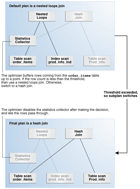
What Oracle does is to make some actual measurements of the number of rows,
apparently during the execution of the query, and then may switch
from one mechanism to the other as it discovers that, whoa, there are lots
of rows to look at.
Optimizer Hints
Oracle supports supplying hints to the optimizer for query execution. Here
are some kinds of hints:
- single-table
- specification of what INDEX to use
- USE_NL to request a Nested Loop join
- multiple-table
- LEADING allows a suggestion of what tables to start with (eg to join
first)
- query block
- UNNEST: applies to nested queries
- STAR_TRANSFORMATION: One table is the center of the "star" and
multiple other tables are accessed relative to the center, but not
relative to one another
- ALL_ROWS
Here are a couple of Oracle's examples. The first is an index suggestion:
SELECT /*+ INDEX (employees emp_department_ix)*/ employee_id, department_id
FROM   employees
WHERE  department_id > 50;
Here is an example of LEADING, which suggests that the join begin with
tables e and j:
SELECT /*+ LEADING(e j) */ *
FROM   employees e, departments d, job_history j
WHERE  e.department_id = d.department_id
AND    e.hire_date = j.start_date;
On what basis might the DBA make such a recommendation?