Comp 346/488: Intro to Telecommunications
Tuesdays 4:15-6:45, Lewis Towers 412
Class 11, Apr 3
Chapter 11, ATM
Chapter 13, congestion control (despite the title, essentially all the detailed information is ATM-specific)
Chapter 14, cellular telephony
Spread Spectrum
9.2: FHSS & Hedy Lamarr /
George Antheil
Both sides generate the same PseudoNoise [PN] sequence. The carrier
frequency jumps around according to PN sequence.
In Lamarr's version, player-piano technology would have managed this;
analog data was used. Lamarr's intent was to avoid radio eavesdropping
(during WWII); an eavesdropper wouldn't be able to guess the PN
sequence and thus would only hear isolated snippets.
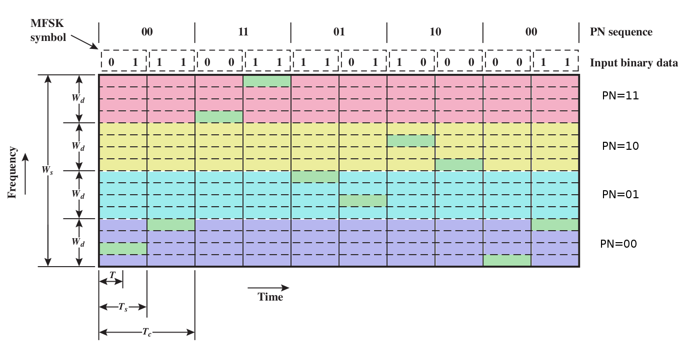
Here's a colorized version of Stallings fig 9.4. The PN sequence
chooses the appropriate broad color band; the four possible values of a
data symbol choose one of the four sub-bands within a broad colored
band.
FHSS
We will use a "pseudo-noise" or pseudo-random (PN) sequence to spread
the frequencies of MFSK over multiple
"blocks"; each MFSK instance uses one block. Each endpoint can compute
the PN sequence, but to the world in between it appears random. For
each distinct PN symbol we will use a band like the MFSK band above,
but we'll have multiple such bands all stacked together, a different
band for each distinct PN symbol.
Tc: time for each unit in the PN sequence
Ts: time to send one block of L bits
slow v fast FHSS/MFSK: Fig 9.4 v 9.5
slow: Tc >= Ts: send >= 1 block of bits for
each PN tick
fast: Tc < Ts: use >1 PN tick to send each
block of bits
feature of fast: we use two or more frequencies to transmit each
symbol; if there's interference on one frequency, we're still good.
Consider 1 symbol = 1 bit case
If we use three or more frequencies/symbol, we can resolve errors with
"voting"
What is this costing us?
9.3: Direct-Sequence Spread Spectrum (DSSS)
Each bit in original becomes multiple bits, or chips. We end up using a lot more
bandwidth for the same amount of information! The purpose: resistance
to static and interference (especially multipath interference).
Same spreading concept as fast FHSS, but stranger.
Basically we modulate the signal much "faster", which spreads the
bandwidth as a natural consequence of modulation. We no longer have a
discrete set of "channels" to use.
Suppose we want to use n-bit spreading. Each side, as before, has
access to the same PN sequence. To send a data bit, we do the following:
- get n bits from the PN sequence
- XOR the data bit with the entire n-bit sequence (that is, if the data
bit is 1, we invert)
- transmit those n bits
Note that we are transmitting n bits in order to communicate one bit. The receiver then:
- receives n bits
- XORs them with the next n bits of the PN sequence
- expects all 0's or else all 1's.
See Figure 9.6.
For every data bit, we will actually receive n bits. Those n bits,
XORed with the appropriate n bits from the PN sequence, should give
either n 0-bits or n 1-bits. A few wrong bits won't matter; we can
simply go with the majority.
Recall that AM band width was proportional to the band width of the
signal. The same thing is happening here: if sending the data 1 bit at
a time needed a band width of B, then sending n bits at a time will
likely need a band width of about nB. Thus, like FHSS, we've greatly
expanded the band width requirement.
Sometimes it is easier to think of the signal as taking on values +1
and -1, rather than 0/1. Then, we can multiply
the data bit by the n-bit PN sequence; multiplication by -1 has the
effect of inverting.
Figure 9.9 shows the resultant spectrum. Because we're sending at a
n-times-faster signaling rate, our spectrum is also n times wider. Why
would we want that? Because jamming noise is likely to be isolated to a
small part of the frequency range; after the decoding process, the
jamming power is proportionally less.
9.4: CDMA
Here, each sending channel is assigned a k-bit chipping code;
each data bit becomes k "chips" (k is often ~128, though in our
examples we'll use k=4 or k=6); these replace the PN sequence (mostly;
see below). Each receiver has the corresponding chipping code. The
chips are sent using
FHSS or DSSS; for DSSS, the sender sendsthe chipping code for a 0-bit and the inverted chipping code for a 1-bit.
As with FHSS and DSSS, one consequence is that data is spread out over a range
of frequencies, each with low power.
Unlike these, however, we are now going to allow multiple transmissions simultaneously,
at least in the forward (tower to cellphones) direction. The signals to
each phone, each with a unique chipping code, are added together and
transmitted together; the receivers need to pick their own data bit out
of the chaos.
basic ideas:
chipping codes: These are the sequences of k bits that we give each user, eg ⟨1,0,1,1,0,0⟩.
The algebra is more tractable if we instead treat 0 as -1, so the code above would become ⟨1,-1,1,1,-1,-1⟩.
dot product: Given two sequences of numbers A = ⟨a1,a2,a3,a4,a5⟩ and B = ⟨b1,b2,b3,b4,b5⟩, the dot product, or inner product, is
A·B = a1*b1 + a2*b2 + a3*b3 + a4*b4 + a5*b5
If our sequences represent vectors in 3-dimensional space (that is, the
sequences have length 3), then A·B=0 if and only if A and B are
perpendicular, or orthogonal.
Suppose we have some pairwise-orthogonal sequences, say A, B, C, and D,
of any dimension (length); that is, A·B = B·C = A·C = A·D = B·D = C·D =
0; any two are perpendicular. Then, if we're given a vector E = a*A +
b*B + c*C + d*D (where a,b,c,d are ordinary real numbers; multiplying a
vector by a real number just means multiplying each component by that
number: 2*⟨3,5,7⟩ = ⟨6,10,14⟩), we can immediately solve for a,b,c,d,
regardless of our geometrical interpretation:
E = a*A + b*B + c*C + d*D
E·A = a*A·A + b*B·A + c*C·A + d*D·A
= a*A·A (because B·A = C·A = D·A = 0)
and so a = E·A / A·A. Similarly we can recover b, c and d. Usually
we'll scale each of the A,B,C,D so A·A = 1, so a = A·E. (We don't do
this below, so A·A = 6.)
The simplest set of orthogonal vectors, or chipping codes, is
⟨1,0,0,0,0,0⟩, ⟨0,1,0,0,0,0⟩, ⟨0,0,1,0,0,0⟩, etc. But it's not the only
set, as we'll see below.
Suppose we have K users wanting to transmit using CDMA. Each user will
be given a vector of 0's and 1's (or -1's and 1's, depending on our
perspective) of length k; this is the user's chipping code. Each user
transmits k "chips" on k frequencies at the same time.
Ideally we use K=k, but in practice K can be rather larger. All the
transmissions add together, linearly (actually, we'll have to adjust
the individual cellphone power levels so that, at the base antenna, all
the signals have about the same power). The transmissions are done in
such a way
that the receiver can extract each individual signal, even though all
the
signals overlap. Similarly, when the base station wants to transmit to
all K users, combines all K bits for each of k positions and transmits
the whole mess; each individual receiver can extract its own signal.
Trivial way to do this: ith sender sends on frequency i only, and does
nothing on other frequencies. This is just FDM, corresponding to the
chipping codes ⟨1,0,0,0,0,0⟩, ⟨0,1,0,0,0,0⟩, ⟨0,0,1,0,0,0⟩, etc. We
don't want to use
this, though.
Example from Table 9.1:
codeA
|
1
|
-1
|
-1
|
1
|
-1
|
1
|
codeB
|
1
|
1
|
-1
|
-1
|
1
|
1
|
codeC
|
1
|
1
|
-1
|
1
|
1
|
-1
|
codeA∙codeB = 0, codeA∙codeC = 0, codeB∙codeC = 2 (using ∙ for "dot product")
userA sends (+1)*codeA or (-1)*codeA
suppose D = data = a*codeA + b*codeB, a,b = ±1
Then D∙codeA = a*codeA∙codeA + b*codeB∙codeA = a*6 + b*0 = 6a; we have recovered A's
bit!
Similarly D·codeB = a*codeA·codeB + b*codeB·codeB = a*0 + b*6 = 6b, and we have recovered B's bit!
Now suppose the transmission D = -1*codeA + 1*codeB + 1*codeC. Can we recover the respective -1, 1 and 1?
combined data D
|
1
|
3
|
-1
|
-1
|
3
|
-1
|
|
codeA
|
1
|
-1
|
-1
|
1
|
-1
|
1
|
|
products w D
|
1
|
-3
|
1
|
-1
|
-3
|
-1
|
sum = -6
|
codeB
|
1
|
1
|
-1
|
-1
|
1
|
1
|
|
products w D
|
1
|
3
|
1
|
1
|
3
|
-1
|
sum = 8
|
codeC
|
1
|
1
|
-1
|
1
|
1
|
-1
|
|
products w D
|
1
|
3
|
1
|
-1
|
3
|
1
|
sum = 8
|
Algebraically, D·codeA = -1*codeA·codeA = -6, because codeA is orthogonal to codeB and codeC
D·codeB = -1*codeA·codeB + 1*codeB·codeB + 1*codeC·codeB = -1*0 + 1*6 +
1*2 = 8. codeB and codeC are not orthogonal but they are "close";
codeB·codeC is "small" relative to 6.
Similarly, D·codeC = -1*codeA·codeC + 1*codeB·codeC + 1*codeC·codeC = -1*0 + 1*2 + 1*6 = 8.
Whenever codeB and codeC appear in the mix, we'll have an extra ±2 in
the mix. But the expected answer is -6, 0, or 6, so if we round to the
nearest such value we'll get the correct result.
Cell phones
analog
The AMPS standard used FDMA (Freq Division Multiple Access): allocates a 30kHz channel to
each call (2 channels!), held for duration of call.
TDMA
digitizes voice, compresses it 3x, and then uses TDM to send 3 calls
over one 30kHz channel.
GSM
form of TDMA with smaller cells, more dynamic allocation of cells. Note
that if everyone talks at once, there might not be enough cells for
all! Data form: GPRS (General Packet Radio Service)
CDMA
sprint PCS, US Cellular, others
code division multiple access: kind of weird. This is a form of "spread
spectrum". Signals are encoded, and spread throughout the band. Any one
bit is sent as ~128 "chips", but chips may be used by multiple senders.
Demultiplexing is achieved because codes are "orthogonal", as above.
This strategy may give good gradual degradation as the number of calls
increases (assuming suitable chipping codes can be found), and good eavesdropping prevention (though not as good as
strong encryption). It also gives excellent bandwidth utilization.
Note that we can only use this orthogonal-chipping-code strategy in the
forward direction (tower to cellphones); for orthogonal codes to work, all the transmissions must be
precisely synchronized. In the reverse direction, we might have had all the
cellphones obey some synchronization protocol, but we don't; instead of
orthogonal codes we use pseudorandom sequences.
Given two random sequences A and B, of length N, the inner product A·B
is typically 0.8*sqrt(N) (unless A=B, in which case A·B = N). We can't
have N cellphones transmit simultaneously and expect the antenna to
decode, but we can have sqrt(N), and furthermore the phones do not have
to be synchronized in any way.
There is some debate about exactly why CDMA works better than TDMA;
theoretically, bandwidth use should be the same. However, the big wins
for CDMA appear to be in avoiding multipath distortion and in frequency
reuse in neighboring cells. If one or two frequencies are affected by
multipath (which is usually very frequency-dependent), the other
frequencies over which CDMA spreads the signal can take up the slack.
Here is Stallings figure 14.2 (at least the N=4 and N=7 cases; the book also illustrates a N=19 example).
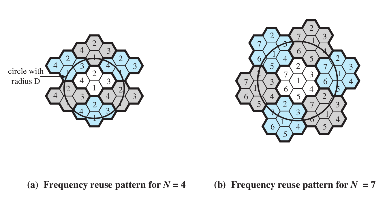
As
for cell reuse, TDMA requires that neighboring cells do not reuse
the same frequencies. CDMA allows adjacent-cell frequency reuse. This
is perhaps the biggest win for CDMA over TDMA; realistic gains are
probably in the range of threefold.
Finally, CDMA may allow for more gradual signal degradation as the service is slightly "oversubscribed"; TDMA simply does not support that.
There is a deep relationship in CDMA between power and bandwidth, but
in a good
way: phones negotiate to use the smallest power for their needs
second reason for CDMA: allows gradual performance falloff with
oversubscription
Chapter 14
Fig 14.1 on cell geometries: a cell diameter is typically a few miles,
though in cities it can be much less
We already considered frequency-reuse patterns over cells, above; here are some other strategies for squeezing out more capacity
- cell sectoring
- cell splitting (works down to ~ 100 m; cells smaller than ~1km
are known as microcells)
- adding frequencies ($$$)
- frequency borrowing
- microcells
Fig 14.6 on finding phones: note that paging is pretty rare; phones
instead "check in" regularly.
Fast (half-wavelength, or 6") fading v slow fading. Here's a
diagram from the IEEE 802.11 wi-fi specification, illustrating the
power-level fluctuations within a room. The wavelength here is about 5
inches, corresponding to the usual spacing between peaks.

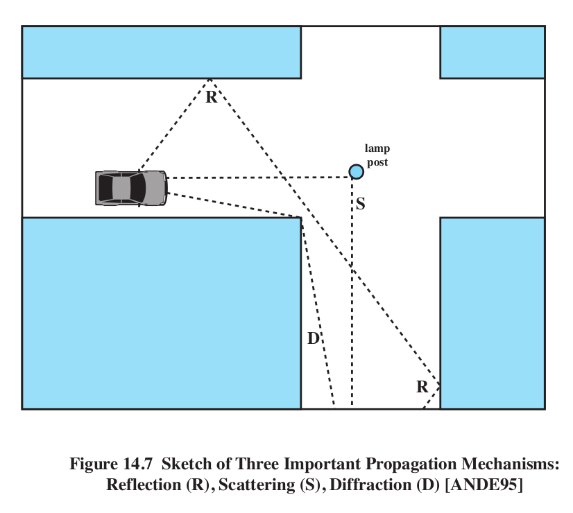
AMPS: FDMA, analog
channel spacing 30kHz!!! This is so big because of multipath distortion (interference)
Multipath distortion:
- reflection
- diffraction
- scattering
Stallings Figure 14.7. Note there is no direct path in this
figure! Normally, the reflected path is the worst offender, when
compared with the direct path.
Phase distortion: multipath can lead to different copies arriving
sometimes in phase and sometimes out of phase (this is the basic cause
of "fast fading").
Intersymbol interference (ISI) and Fig 14.8. Pulses might be sent 1
unit apart, but multipath distortion might create "echo" pulses at
times, say, 0.3, 0.5 and 0.9 units following the original pulse. That
last echo is likely to interfere with the next data pulse.
Note that CDMA requires good power control
by the phones so that all signals are roughly equal when received at
the cell tower. Phones all adjust signal strength downwards if received
base signal is
stronger than the minimum.
Go through Andrews presentation at http://users.ece.utexas.edu/~jandrews/publications/cdma_talk.pdf
- Walsh codes at base station (below)
- PN codes in receivers (because we no longer can guarantee
synchronization)
- Frequency reuse issues
SMS (text messaging)
This originated as a GSM protocol, but is now universally available
under CDMA as well, and these can be transmitted within SS7. Basically, the message piggybacks on "system" packets.
Walsh Codes
How are we going to get orthogonal codes? I tried (using brute-force
search) to find a third code orthogonal to the length-6 A&C above or to
A&B; there are none!
If k is a power of 2, we can do this with Walsh codes. We will create a k×k matrix of +1 and -1 where all the rows are orthogonal. This is done recursively.
k=1: the matrix is just [+]
k=2: the matrix is
k=4:
+
|
+
|
+
|
+
|
+
|
−
|
+
|
−
|
+
|
+
|
−
|
−
|
+
|
−
|
−
|
+
|
k=2r. Let M be the Walsh matrix of size 2r-1. Arrange four copies of M in a 2r × 2r matrix as follows, where −M is the result of flipping every entry in M:
Note that this is what we did to go from k=1 to k=2 above, and from k=2 to k=4.
Erlang model
Suppose we know the average
number of simultaneous users at the peak busy time (could be calls
using a trunk line, could be calls to help desk). We would probably
figure that at least some of the time, the demand might be higher than
average. How many lines do we actually need?
To put this another way, suppose we flip 200 coins. The average number
of heads is 100. What are the odds that in fact we get less than or
equal to 110 heads? Or, to put it in a slightly more parallel way,
suppose we keep doing this. We want to reward every head-getter, 99% of the time.
How many rewards do we have to keep on hand?
One parameter is the acceptable
blocking rate:
the fraction of calls that are allowed to go unconnected (ie that receive the fast-busy or "reorder" signal). As this rate
gets smaller, the number of lines needed will increase.
Example: how
many lines do we need to handle a peak rate of 100 calls at any one
time (eg 2,000 users each spending 5% of the day on the phone), and a
maximum blocking rate of 0.01%?
(From http://erlang.com/calculator/erlb
and my own program)
We assume that calls for which a line is not available are BLOCKED, not
queued. (There is an alternative Erlang formulation for the queued model.) Here is a table; the call rate is the average number of simultaneous calls, and allowed blocking is the fraction of calls that can be blocked.
call rate
|
allowed blocking
|
lines needed
|
excess
|
10
|
0.01
|
18
|
180%
|
20
|
0.01
|
30
|
150%
|
50
|
0.01
|
64
|
128%
|
100
|
0.01
|
118
|
118%
|
180
|
0.01
|
201
|
111%
|
200
|
0.01
|
221
|
110%
|
500
|
0.01
|
526
|
105%
|
1000
|
0.01
|
1029
|
103%
|
To a reasonable approximation, if we have 200 lines, we can handle ~180
calls.
Here's a table where the blocking rate is 0.001:
call rate
|
allowed blocking
|
lines needed
|
excess
|
10
|
0.001 |
21 |
210% |
20
|
0.001 |
35 |
175% |
50
|
0.001 |
71 |
142%
|
100
|
0.001 |
128 |
128% |
180
|
0.001 |
216 |
120%
|
200
|
0.001 |
237 |
119% |
500
|
0.001 |
554 |
111% |
1000
|
0.001 |
1071 |
107% |
The number of lines needed is always greater than the average peak rate. The
question is by how much.
As allowed blocking rate goes down, the number of lines needed goes up, for
the same call rate.
Also, as the call rate goes up, the number of extra lines goes up but the percentage of extra lines needed goes DOWN, due
to the "law of large numbers"
ATM: Asynchronous Transfer Mode
versus STM: what does the "A" really mean?
Basic idea: virtual-circuit networking using small (53-byte) fixed-size
cells
Review Fig 10.11 on large packets v small, and latency. (Both sizes give equal
throughput, given an appropriate window size.)
basic cellular issues
delay issues:
- 10 ms echo delay: 6 ms fill, ~4 ms for the rest
- In small countries using 32-byte ATM, the one-way
echo delay might be 5 ms. Echo cancellation is not cheap!
Supposedly (see Peterson & Davie,
wikipedia.org/wiki/Asynchronous_Transfer_Mode) smaller countries wanted
32-byte ATM because the echo would be low enough that echo cancellation
was not needed. Larger countries wanted 64-byte ATM, for greater
throughput. 48 was the compromise. (Search the WikiPedia article for
"France".)
150 ms delay: threshhold for "turnaround delay" to be serious
packetization: 64kbps PCM rate, 8-16kbps compressed rate. Fill times: 6
ms, 24-48 ms respectively
buffering delay: keep buffer size >= 3-4 standard deviations, so
buffer underrun will almost never occur. This places a direct
relationship between buffering and jitter.
encoding delay: time to do sender-side compression; this can be significant but usually is
not.
voice trunking (using ATM links as trunks) versus voice switching
(setting up ATM connections between customers)
voice switching requires support for signaling
ATM levels:
- as a replacement for the Internet
- as a LAN link in the Internet
- MAE-East early adoption of ATM
- as a LAN + voice link in an office environment
A few words about how TCP congestion control works
- window size for single connections
- how tcp manages window size: Additive Increase / Multiplicative
Decrease (AIMD)
- TCP and fairness
- TCP and resource allocation
- TCP v VOIP traffic
ATM
basic argument (mid-1980s): Virtual circuit approach is best when
different applications have very different quality-of-service demands
(eg voice versus data)
why cells:
- reduces packetization (fill) delay
- fixed size simplifies switch architecture
- lower store-and-forward delay
- reduces time waiting behind lower-priority big traffic
no-reordering rule, and its consequences