Comp 346/488: Intro to Telecommunications
Tuesdays 4:15-6:45, Lewis Towers 412
Class 7, Feb 28
Reading (7th -- 9th editions)
Chapter 10: 10.1, 10.2, 10.3
Latest fun & games with Asterisk:
Instead of having callers wait in their phone queues on a FIFO basis,
have them play games. If they win, they move ahead in the queue. If
they lose, they move backwards. I'm still trying to find out implementation details.
SONET
Good reference: sonet_primer.pdf
Sonet is said to be truly synchronous:
timing is supposed to be exact, to within ±1 byte every several frames.
Bit-stuffing (pulse stuffing) was seen by the telecommunications
industry as a major weakness in the T-carrier system, introducing more
and more wasteful overhead as the multiplexing grew. The core issue is
that when you combine several "tributaries" into one larger data
stream, your big stream needs extra capacity to be able to handle
speedups and
slowdowns in the inputs.
SONET was an attempt to avoid this problem.
First look at SONET hierarchy: Stallings Table 8.4 (largely reproduced
below)
STS-1/OC-1
|
|
51.84 Mbps
|
STS-3/OC-3
|
STM-1
|
155.52 Mbps
|
STS-12/OC-12
|
STM-4
|
622.08 Mbps
|
STS-48/OC-48
|
STM-16
|
2488.32 Mbps
|
STS-192
|
STM-64
|
9953.28 Mbps
|
STS-768
|
STM-256
|
39.81312 Gbps
|
STS-3072
|
|
159.25248 Gbps
|
STS = Synchronous Transport Signal
OC = Optical Carrier
STM = Synchronous Transport Mode [?]
Note that each higher bandwidth is exactly
4 times the previous (or 3 for the first row). There is no bit
stuffing, though there is a
mechanism to get ahead or fall behind one byte at a time.
basic SONET frame (Stallings v9 Fig 8.11)
-
Transport overhead, path overhead
- framing bytes: A1, A2 0xF628
- multiplexing number: STS-ID
- E1, E2, F1: special header-only voice lines ("orderwires")
- H1-H3: frame alignment
- one of these allows byte stuffing, and/or frame drift.
A1
|
A2
|
J0
|
J1 |
data cols 4-29
|
J1 |
data cols 31-58
|
J1
|
data cols 60-90
|
|
E1
|
|
|
|
|
|
|
|
|
|
|
|
|
|
|
|
|
H1
|
H2
|
H3
|
|
|
|
|
|
|
|
|
|
F2
|
|
|
|
|
|
|
|
|
|
|
|
|
|
|
|
|
|
|
|
|
|
|
|
|
|
|
|
|
|
|
|
|
|
|
E2
|
|
|
|
|
|
|
The payload envelope, or SPE, is the 87 columns reserved for path
data. The SPE can "float"; the first byte of the SPE can be any byte in
the non-overhead part of the frame; the next SPE then begins at the
corresponding position of the next frame. (The diagram above does not show a floating SPE.) This
floating allows for the
data to speed up or slow down relative to the frame rate, without the
need for T-carrier-type "stuffing".
SPEs are generally spread over two consecutive frames. It is often
easier to visualize this if we draw the frames aligned vertically.
The first column of the SPE is the path
overhead; columns 30 and 59 are also reserved. In the diagram
above, these are the columns beginning with J1. Total data columns: 84.
Note that the path-overhead columns mean that the longest run of bytes
before a 1-bit is guaranteed is about 30; the SONET clocking is usually
accurate enough to send 240 0-bits (30 bytes) and not lose count.
SONET resynchronization
However, sometimes SONET does lose count, and has to re-enter the
"synchronization loop". This can involve a delay of a few hundred
frames (~40-50 ms). Packets with the "wrong" kind of data (resulting in
long runs of 0-bits after scrambling) are often the culprit; carriers
don't like this.
Frame synchronization is maintained by keeping track of the fixed-value
framing bytes A1A2. If these are ever wrong (ie not 0xF628), we go into
the resynchronization loop. Every bit position is checked to see if it
begins the 16-bit sequence 0xF628. If it does, we check again one full
frame later. Over a certain number of frames we decide that we are
synchronized again if we keep seeing 0xF628 in the A1A2 position.
Note that synchronization involves finding the byte boundaries as well
as the frame boundaries.
0xF628 is 1111 0110 0010 1000. It is straightforward to build a
finite-state machine to recognize a successful match, while receiving
bits one at a time.
There is no natural byte framing in SONET. (Actually, there is no natural byte framing on any synchronous serial line.)
8000
SONET frames are always sent at 8000 frames/sec (make that 8000.0000
frames/sec). Thus, any single byte position in a frame can serve, over
the sequence of frames, as a DS0 line, and SONET can be viewed as one
form of STDM.
STS-1: 9 rows × 90 columns × 8 bits/byte × 8 frames/ms = 51840 b/ms
frame rate
Data rate: 9 rows × 84 columns × 8 × 8 = 48.384 mbps
DS-3 rate: 44.7 mbps
STS-3: exactly 3 STS-1 frames
An end-to-end SONET connection is essentially a "virtual circuit",
where the sender sends STS-1 frames (or larger) and the receiver
receives them. These frames may be multiplexed with others inside the
network. These frames are themselves often the result of multiplexing
DS lines and packet streams.
SONET connections are divided into the following three categories,
depending on length:
- a section is a single
run of fiber between two repeaters.
- a line is a series of
sections between two multiplexers.
- a path is anything longer
Stuffing
The SPE arrival rate can run slower than the 8000 Hz frame rate, or
faster. Stuffing is undertaken only at the Line head, ie the point
where multiplexing of many SPEs onto a single line takes place.
Positive stuffing is used when
the SPEs are arriving too slowly, and so an extra
frame byte will be inserted between occasional SPEs. The SPE-start J1
byte will slip towards the end of the frame. Some bits in the H1-H2
word are flipped to indicate stuffing; as a result, in order to ensure
a sufficient series of unflipped H1-H2 words, stuffing is allowed to
occur only every third frame.
Negative stuffing is used when
the SPEs are arriving slightly too fast. In this case, the pointer is
adjusted (again with some bits in the H1-H2 word flipped to signal
this), and the extra byte is placed into the H3 byte. The J1 SPE-start
byte moves towards the start of the frame ("forward").
Note that negative stuffing cannot occur twice, but never has to.
Stuffing is only done at line entry. If a line is ended, and
demultiplexed, and one path is then remultiplexed into a new line, then
stuffing begins all over again with a "clean slate".
The fact that the SPE can "slip back" (or creep forward) in the frame
means that once we handle a byte of slip/creep, we're done with it. It
doesn't accumulate, except as an accumulation of slip/creep.
Virtual Tributaries
An STS-1 path can be composed of standard "substreams" called virtual
tributaries. VTs come in 3-column, 4-column, 6-column, and 12-column
versions.
If we multiplex 4 DS-1's into a DS-2, and then 7 DS-2's into a DS-3,
then the only way we can recover one of the DS-1's from the DS-3 is to
do full demultiplexing. Virtual tributaries ensure that we can package
a DS-1 into a SONET STS-1 channel and then pull out (or even replace)
that DS-1 without doing full
demultiplexing.
You can lease a whole STS-N link, a SONET virtual tributary, or a DS-1
or DS-3 line.
SONET and clocking
This is very synchronous.
All clocks trace back to same atomic source. For this reason, clocking
is NOT a major problem. Data is sent NRZ-I, no stuffing.
Strictly speaking, all the SONET equipment in a given "domain" gets its
clock signal from a master source for that domain. All equipment should
then be on the same clock to within ± 1 bit.
The stuffing mechanism described above is for interfaces between "clock domains", where
there may be slight differences in timing. When this occurs, we are
back to a plesiochronous setting.
NOTE: the rectangular layout
guarantees at most 87 bytes before a nonzero value; XOR with a fixed
pseudorandom pattern is also used. (Actually, the max run of 0's is 30
bytes, because of the "fixed" SPE columns.)
SPE path overhead bytes:
J1: over 16 consecutive frames, these contain a 16-byte "stream
identifier"
B3: SPE parity
C2: flag for SPE content signaling (technical)
G1: round-trip path monitoring ("path status")
F2: path orderwire
H4:
Z3, Z4, Z5: path data
Note that the J1 "stream identifier" SPE byte is the closest we have to
a "stream address". SONET streams are more like "virtual circuits" than
packets (a lot more like!): senders "sign up" for, say, an STS-1
channel to some other endpoint, and the SONET system is responsible for
making sure that frames sent into it at the one end come out at the
right place at the other end. Typically the input to an STS-1 channel
is a set of DS-1/DS-3 lines (at most one DS-3!), or perhaps those mixed
with some ATM traffic.
An orderwire is a circuit used
for
management and maintenance. In the SONET orderwire examples below,
the orderwire circuits in the path overhead and transport overhead are
DS0, making them suitable for voice. But there is no
requirement that voice actually be used.
IP over SONET
This can be done IP → ATM → SONET, or else using POS (Packet Over
SONET).
The IP packet is encapsulated in an HDLC packet, using HDLC bit
stuffing as needed; we don't care about packet-size expansion because
there are no tight timing constraints on IP packet transmission. We
then lay the results out in the data part of a SONET
frame, using the Point-to-Point Protocol (PPP) to supply signaling
overhead. During idle periods, we send the HDLC start/stop symbol (0111
1110) bytes, which
might not in fact end up aligned on byte boundaries of the SONET frame
due to HDLC bit-stuffing. The PPP/HDLC combination works over any
bitstream.
Note that SONET bitstreams do have byte boundaries, but there are no
byte boundaries in the T-carrier hierarchy. The Packet Over SONET
approach simply ignores the underlying SONET byte boundaries.
Back to chapter 10
Revisit Figure 10.2, on plugboard switching. But now envision the
switches as electronic, and the trunk lines as bundles of STDM channels
rather than copper wires.
Another switch picture can be found in Fig 10.4. The "Full-duplex lines
to attached devices" at the left should be thought of as channels.
Fig 10.3 shows a simple call setup.
Between the customer premise and the local office, in-band (or inchannel) signaling is likely used:
the voice line carries the pulse or DTMF (touch-tone) signals. There is
in most cases no alternative signaling path!
Between offices it is a different story. Once upon a time, in-band
signaling was once used there too. This meant that as each channel in the
end-user-to-end-user path was allocated, the setup signaling would
traverse that path to the next switch in the system; the call-setup
signaling followed the same path through the network as the voice data
to come. Another term for this is associated
signaling: the signal path is associated
with (that is, identical to!) the data path.
This has drawbacks. For one thing, it is slow, and there can be no
global allocation of the channels that make up the end-user-to-end-user
path. The SS7 system allows out-of-band
signaling, or common-channel signaling ("common" here means that the signaling packets all use one separate channel/network in common, not in common with the voice circuits):
all the switches are connected via a packet-switched channel or network
that is logically separate from any of the channels that link
adjacent switches. This allows communication between the endpoints to
begin even before any channels are allocated; it also allows a global
channel-allocation strategy.
Out-of-band signaling can also be associated, if the signaling data
follows more-or-less the same path as the voice circuits. More likely
the signaling is disassociated, meaning that unrelated paths are used. Sometimes the term information plane is used to describe the network map that the voice channels use; the control plane is the map of the setup network.
Blue boxes and in-band signaling
In the days before SS7 (in which the signaling data is communicated
through a parallel packet-switched network), switch signaling was done
over the same voice lines that the call would eventually use. Idle
trunk lines would have a 2600 Hz tone transmitted both ways. Trunk
links were allocated to a call on a hop-by-hop basis starting from the
caller: each switch would (a) stop sending the 2600 Hz tone, and (b)
transmit the dialed number as a sequence of DTMF (touchtone) digits.
The receiving switch would save the digits, allocate a trunk line to be
the next link on the path, and repeat the process. The final switch
would simply complete the call to the destination subscriber using that
subscriber's "local loop". The first switch on the path would be
responsible for billing. To tear down the call, the first switch would
send the 2600-Hz tone again to tell the trunk segments they were idle.
So, to place a call, you first needed to dial a local number:
one that would involve at least one trunk segment, and which was cheap
(ie either semi-local (but still involving one trunk segment), or an
800-number). Billing would commence at that rate. You then sent the
2600-Hz tone, which would make all the trunk segments go idle. The
first switch, however, not having been informed of any disconnection,
still had you connected to the first trunk on the path, which we'll
call trunk1.All subsequent trunk segments would actually be released.
You would then send the long-distance number, in DTMF form. The first
trunk would get these digits and assume they were part of legitimate
call-routing; the call-setup process would run as normal. Note that a real call to that long-distance number might not use the trunk1 link at all, but that it did not matter.
At this point you were connected to the long-distance number, but paying for the local number.
This is not the only disadvantage to in-band signaling; another was
that the path had to be allocated on a purely hop-by-hop basis. And the
security hole might have been closeable by other means. Still, the
blue-box problem was a significant one.
Overview of circuit-setup process
Connections are made between A and a, B and B, etc. Links between
adjacent switches are really large bundles of "bearer circuits", ie DS0
channels.
S1[A,B]
\
\
\
S3[] ------------------------------------ S4[]
------------------------------- S5[b,c,d,e,f]
/
/
/
/
/
/
S2[C,D]
S6[E,F,a]
For each switch, the endpoints directly connected to it are in
brackets: A-F connected respectively to a-f. The S3-S4 and S4-S5 links
are second-level multiplexes. We demultiplex at S3, S4, and S5, and a
given channel from the S3-S4
line is connected to a different channel on the S4-S5 line. Those
channel connections are what the circuit setup process must create.
Circuits may be on-demand, as
in phone calls, or permanent,
as in something a subscriber (eg an ISP) has contracted for on a
permanent basis.
Circuit-setup can take inefficient paths, causing early blocking. Consider the following diagram of endpoints A and B and switches S1 and S2.
        A
      //  \
     //    \
    S1-----S2
     \\    /
      \\  /
        B
This arrangement can support three paths from A to B: two taking the
route A-S1-B and one taking the route A-S2-B. But suppose we create a
path A-S1-S2-B, outlined in red above. Ath this point, only one more
path from A to B is possible (the blue one). The red zigzag path has blocked the third
path.
Switches
T-1, T-3, and SONET circuit-switching
A T-3 can be demultiplexed into its constituent
DS-2's (rare), DS-1's, or DS-0's.
A SONET STS-12 can be demuxed into all sorts of
things, eg
one STS-4
eight STS-1's
five of them are really
DS-3's
one of them is a plain
IP-over-SONET
two are a "double-sized"
IP-over-SONET, at 2xSTS-1 rate
Any given SONET line (portion
with no change in multiplexing) is a pure circuit-switched link.
Switching is done where the lines join together to form a path.
In general, in the phone system they like to avoid "full
demultiplexing" where possible, when dealing with DS-n lines. That's
because demultiplexing involves some overhead for these. For SONET, the
overhead is negligible; we can replace a single DS-0 in an STS-48 with
relative ease.
Crossbars
For connecting channels, the crossbar switch can be used (Stallings Fig
10.5). Crossbars were once made with electromechanical relays at each
crossing point; they can also be made with electronic switches.
Crossbars allow any input line to be connected to any output line.
Furthermore, if the crossbar is N×N, and we have any (permutation) map
f:{1,2,3,..,N} ⟶ {1,2,3,...,N}, we can connect input i to output f(i);
that is, there are never any "conflicts" or internal blocking.
However, crossbars are expensive.
So in the real world multi-stage
switches (Stallings Fig 10.6) are much more common:

Note, however, that this switch blocks.
We cannot connect 2 in upper input half to 3 in upper output half,
given the existing connections. In general, we cannot have more than
two connections at a time.
Networks usually tolerate some degree of blocking.
A crossbar switch is an example of "space-division multiplexing"
These things are called "switch fabrics"
The inputs to these switches are the mux/demux channels.
Clos switches
This is the category of switch in Stallings' Fig 10.6. The concept
itself
was first described in a 1953 Bell Labs paper by Charles Clos. The
general idea is the three-column "sparse crossbar" (in Fig 10.6, r=2, m=2, n=5)
Column 1: r many n×m crossbars. Total inputs: rn; total outputs: rm
Column 2: m many r×r crossbars. Total inputs: rm; total outputs: rm
Column 3: same as Column 1, wired in reverse (that is, r many m×n crossbars; total inputs: rm, total outputs: rn).
The m outputs of each Column 1 n×m crossbar are connected to every one
of the r×r Column 2 crossbars.
Any connection is uniquely determined by its entry port (which port on
which Column 1 crossbar), its Column 2 crossbar, and its egress port.
Note that the specific port on the Column 2 crossbar is uniquely
determined by the wiring; we do not have to specify it.
All this replaces one large N×N crossbar, where N=nr.
Suppose we take n≃m≃r. Then n ≃ N1/2. The size of the Clos
configuration is = 2nmr + nr2 ≃ 3n3 ≃ 3N3/2.
The savings in space over the full crossbar is N1/2/3. For
N=1000 this is a factor of 10; for N=10,000 it is a factor of 30.
Fact 1: if m ≥ 2n−1, then the
switch is completely nonblocking:
any
free input on the left can be connected to any free output on the right.
Proof: Here's the simpler case where m = 2n−1; the general case is the
same, but you use inequalities.
Consider the left and right-hand n×m and m×n crossbars that we wish to
connect: these are the entry and egress crossbars. Each has at most n−1
active inputs, and thus at most n−1 active outputs, and thus at least
m−(n−1) free outputs. The
hypothesis means m−(n−1) = m−n+1 = 2n−1−n+1 = n, so there are at least
n free outputs.
The entry crossbar thus has at least n free connections to column 2,
and there are similarly n free connections from column 2 to the egress
crossbar. We need to show that there is at least one column 2 crossbar
has a free connection to both
the entry and egress crossbars. But this has to happen, because there
are m = 2n−1 column 2 crossbars, and n connected to the entry crossbar
and n connected to the egress. If there were no overlap in the set of
column-2 crossbars connected to the entry and the set of column-2
crossbars connected to the egress, then there would have to be at east
2n column-2 crossbars in all, which there are not.
Fact 2: if m≥n, then any input
can be connected to any output provided
that we are allowed to reroute
some existing connections to a different
Column-2 crossbar to make room. Note that all we have to specify for an
existing connection is which Column-2 crossbar it is to use.
Blocking/rerouting example 1: Nine 3×3 crossbars arranged in a 3x3 pattern. There are
three existing connections, designated by which crossbar in column 1
connects to which crossbar in column 3 (actual ports don't matter). Let
us refer to the middle column crossbars as M1, M2, and M3.
- row 1 to row 2, via M1
- row 2 to row 1, via M2
- row 3 to row 1, via M3
We now wish to add one new connection from row 1 to row 1; this should
be doable, as the row 1 column 1 switch has one of its three inputs in
use, and the row 1 column three switch has two of its three outputs in
use.
However, we cannot use any of the column 2 switches to complete the
circuit: for M1, the line to the entry switch is blocked, and for M2
and M3, the line to the egress switch is blocked.
The call becomes possible if we move connection 1 so that it uses M2,
freeing M1 for the new connection. Or we can move connection 2 so that
it uses M1, freeing M2 for the new connection.
Blocking/rerouting example 2: Consider the example below, from http://en.wikipedia.org/wiki/Nonblocking_minimal_spanning_switch.
Connections A-A (red), B-B (green), C-C (orange) and D-D (blue) have
been made, and we want to add a connection from E to E. However, we're
stuck. If the middle column of switches are numbered 1,2,3,4 from top
to bottom, then E can only connect to 3 and 4. However, 3's output to
the E switch in the third column is in use (orange), and 4's output
(blue) is also in use.

However, we can move a call:
there are several possibilities. One is to move the B-B (green) path
from middle switch 2 down to 3, freeing up the E-E connection to use
middle switch 2. Another is to move the blue D-D connection up. If we
move it to middle switch 2 then the E-E connection is still blocked,
but we can move it to middle switch 1 and then we can connect E and E
through middle switch 2.
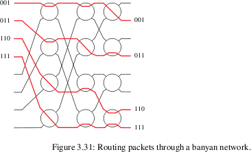
Banyan switches
Banyan switches can replace a full N×N crossbar with N/2*log(N)
switches, arranged in (N/2) rows and log(N) columns. Each input,
however, must be prefixed with
a binary routing string
(of length log(N)) representing the output port. Each switch element
has two inputs and two outputs. The element uses the first bit of the
prefixed routing string to decide which output to use.
Banyan networks many involve collisions, in principle. In practice, a
mesh can be constructed so that collisions never occur, so long as the
inputs that enter the switch fabric simultaneously are sorted by their routing strings: eg
001, 101, 110, 111.
Virtual-circuit packet-switched routing
We don't usually use
the word "virtual" for TDM, though TDM circuits are in a sense virtual.
But "virtual circuit switching" means using packets to simulate circuits.
Note that there is a big difference between circuit-switched
T-carrier/SONET and any form of packet-based switching: packets are
subject to fill time. That is,
a 1000KB packet takes 125 ms to fill, at 64 Kbps, and the voice
"turnaround time" is twice that. 250 ms is annoyingly large. When we
looked at the SIP phone, we saw RTP packets with 160 B of data,
corresponding to a fill time of 20 ms. ATM (Asynchronous Transfer Mode)
uses 48-byte packets, with a fill time of 6 ms.
Datagram Forwarding
Routers using datagram forwarding each have ⟨destination, next_hop⟩
tables. The router looks up the destination of each packet in the
table, finds the corresponding next_hop, and sends it on to the
appropriate directly connected neighbor.
These tables are often "sparse"; some
fast lookup algorithm (eg hashing) is necessary. The IP "longest-match"
rule complicates this. For IP routing, destinations represent the network portion of the address.
How these tables are initialized and maintained can be complicated, but
the simplest strategies involve discovering routes from neighbors.
Often a third column, for route cost, is added.
drawback: cost proportional to # of nodes
first look at virtual circuit goals:
- small cells
- small header
- low per-packet cost
- still packet-switched!
Packet size figure: 10.14 (7th), 10.11(8th, 9th)
Uniformity of delay (ie jitter) is a separate issue, but is often worse with datagram switching
virtual circuits
Call Request; sets up route; the route between two endpoints must be set up in advance, and is encoded by switch state.
Each switch has a table of the form ⟨vciin, portin, vciout, portout⟩
vci+port are treated as a contiguous string of bits, small enough to use as an array index, which is very fast!
Entries are typically duplicated, so given the vci+portin we can look up vci+portout, and given vci+portout we can find vci+portin.
This allows bidirectionality.
All this allows very compact lookup tables, generally faster on a per-packet basis than datagram forwarding but requires setup.
smaller addresses / smaller headers
Addresses identify the PATH, not the DESTINATION
PATH address is VCI, which is not globally unique!! VCIs are local, leading to fewer bits
What are virtual circuits good for?
- fast routing
- low per-packet overhead
- addresses are small!
=> still efficient even when packets are small!
Also, can be BIDIRECTIONAL
Remarks about datagram-forwarding table maintenance
continue with VC example
- assignment of link addresses
- next-hop basis for connection setup
- single-point-of-failure vulnerabilities
- supports billing