More SQL
Here is a quick summary of SQL
Here is a slightly-less-quick introduction.
This file contains most of the examples from EN6 chapter 5 / EN7 chapter 7,
and related examples from other sources.
Self joins
A tricky foreign-key constraint
Union and intersection
Join examples in terms of keys
Outer joins
Nulls
Simpler nested queries
Grouping functions
GROUP BY
Correlated nested queries
Exists and Unique
ALL (as universal quantification)
EXCEPT
HAVING
Views
Triggers
Why is SQL sometimes hard?
Basically, it's hard because it is a non-imperative language:
you don't issue a sequence of commands. Instead, you write a single
big expression. It's hard to visualize big expressions, and hard to
test them incrementally. Nested queries do seem to help in this regard.
(Actually, the data types of SQL are tables, and you can in
fact save a table in a "table variable". But this is rare.)
Perhaps because of this non-imperative nature of the language, it is
relatively easy to read several SQL examples and still have trouble
knowing where to start when trying to write one from scratch.
What Joins Do
Consider a simple join example, in which we print each employee name
together with the name of the employee's department:
select e.fname, e.lname, d.dname from
employee e join department d on e.dno = d.dnumber;
Oone can think of e and d as "cursors", or row variables, representing rows
in the respective tables employee and department. Linear search through the
employee table , as in the SQL example
select e.lname, e.salary from employee e
where e.salary >= 30000;
might be represented by the following java-like loop, showing a linear
search through the table:
for (e
in employee) {
if (e.salary >= 30000) {
print(e.lname, e.salary)
}
}
Now let's write this for the above join; here we get a nested loop and
quadratic runtime (specifically, O(nm), where n=employee.size() and
m=department.size())
for (e in employee) {
for (d in department) {
if (e.dno == d.dnumber) {
print(e.fname, e.lname, d.dname)
}
}
Clearly, for triple joins over large databases, performance is an issue.
This is addressed two ways: query optimization, to
eliminate "obvious" inefficiencies, and internal indexes.
The primary key defines a candidate for indexing, though not all indexing is
on key fields.
Self-join
Without a join, all you can look at is one row at a time of one
table. When we join EMPLOYEE and DEPARTMENT, eg
select e.lname, d.dname from employee e,
department d where e.dno = d.dnumber;
we are looking at one row at a time of each table, but two tables. The
DEPARTMENT table is being used here to "extend" the EMPLOYEE table: each
employee record now has additional attributes from DEPARTMENT.
Suppose we want to print a list of all employees and their supervisors.
Here's the approach we might take:
select e.fname, e.lname, s.fname, s.lname
from employee e join employee s on e.super_ssn = s.ssn;
The idea here, in terms of cursors, is for e to traverse linearly the
employee table. For each employee, we get e.super_ssn, and then use s to
traverse the same table, looking for a row with s.ssn = e.super_ssn.
Each record in the result is a combination of two rows
of table EMPLOYEE, so a join is necessary.
In terms of table extension, the EMPLOYEE table is being "extended" to
include additional attributes about supervisors besides just super_ssn.
This particular example is much more readable if we relabel the supervisor
columns in the output
select e.fname, e.lname, s.fname AS
super_fname, s.lname AS super_lname
from employee e join employee s on e.super_ssn = s.ssn;
Note that the AS here is not optional, and plays a rather different role
than the AS that can be used in the FROM section (from employee AS e,
employee AS s).
A tricky foreign-key constraint
Let's try to create a foreign key constraint to require that any
project.plocation must appear as a dept_locations.dlocation:
alter table project ADD constraint
        FK_project_dept_locations foreign key (plocation) references
        dept_locations(dlocation);

        alter table project drop foreign key
FK_project_dept_locations;
-- to undo
(Do you think this is actually a reasonable rule?)
But this fails, because dlocation is not a key of
dept_locations (actually, this is a slight oversimplification; see below).
Foreign-key constraints are already a performance hit; non-key lookups are
in principle quite a bit less efficient. I get:
MySQL: ERROR 1215 (HY000): Cannot add
foreign key constraint [not very helpful!]
Postgres: ERROR: there is no unique constraint matching given keys
for referenced table "dept_locations"
What the Postgres error message means is that dept_locations.dlocation --
the "referenced table" -- is not a key. MySQL is slightly more
relaxed; its actual concern is that table dept_locations does not have an index
on the dlocation column. The important thing is for the RDBMS to be able to
verify a given FK constraint quickly, by using an index on the parent table.
If the FK reference is to the parent table's primary key, then the index is
automatic as MySQL and Postgres create an index on the primary key for every
table.
More at http://dev.mysql.com/doc/refman/5.0/en/create-table-foreign-keys.html
MySQL
To create an index (simplified version), use
create index indexname on tablename(indexcolumn);
create index dloc_index on dept_locations(dlocation);
drop index dloc_index on dept_locations;
At this point, the above "alter table ..." command works under MySQL, though
it still does not work under Postgres.
Postgres
Here is the Postgres
rule:
A foreign key must reference columns that
either are a primary key or form a unique constraint. This means that the
referenced columns always have an index (the one underlying the primary
key or unique constraint); so checks on whether a referencing row has a
match will be efficient.
That is, the actual requirement is that the referenced attribute (or set of
attributes) be a key, though the reason given for this is so that
there is an index (which we could in principle add separately).
Here is one workaround:
create table legal_locations (
location varchar(15)
primary key
);
insert into legal_locations (select distinct dlocation from
dept_locations);
-- no "values"
alter table project ADD foreign key (plocation) references
legal_locations(location);
alter table dept_locations ADD foreign key (dlocation) references
legal_locations(location);
To remove these:
show create table project;
alter table project DROP foreign key project_ibfk_2;
show create table dept_locations;
alter table dept_locations DROP foreign key dept_locations_ibfk_1;
But there is in fact a better way: a two-column
foreign-key constraint. This assumes that what we want is for the
(plocation,dnum) pair in the project table to match a pair
(dnumber, dlocation) from dept_locations. If this is what we want, we can do
this:
alter table project add constraint
        FK_project_dept_locations foreign key (plocation, dnum) references
        dept_locations(dlocation, dnumber);
alter table project drop constraint FK_project_dept_locations;
Here we don't have to worry about the key because (dnumber,dlocation) is
a key for dept_locations. With the above constraint in place, we cannot add
a project to dept 1 in Stafford:
insert
into project values ('partythings', 34, 'Stafford', 1);
delete from project where pnumber = 34;
Names of employees
who have worked on project 2 OR project 3:
select e.fname, e.lname , w.pno from
employee e join works_on w on e.ssn = w.essn
where w.pno = 2 or w.pno =3;
Alternatively:
(select e.fname, e.lname, w.pno from
employee e join works_on w on e.ssn = w.essn where w.pno = 2)
union
(select e.fname, e.lname, w.pno from employee e join works_on w on e.ssn =
w.essn where w.pno = 3);
Names of employees who have worked on
project 2 AND project 3.
This one is harder! If we change the or
above to and, we get nobody.
select e.fname, e.lname, w.pno from employee e join works_on w on e.ssn =
w.essn where w.pno = 2;
+----------+---------+-----+
| fname |
lname | pno |
+----------+---------+-----+
| John |
Smith | 2 |
| Franklin | Wong
| 2 |
| Joyce | English
| 2 |
+----------+---------+-----+
select e.fname, e.lname, w.pno from employee e join works_on w on e.ssn =
w.essn where w.pno = 3;
+----------+---------+-----+
| fname |
lname | pno |
+----------+---------+-----+
| Franklin | Wong
| 3 |
| Ramesh | Narayan
| 3 |
+----------+---------+-----+
From looking at these, it is clear that Franklin Wong has worked on both.
Attempt 1: use the intersect operator. For this to work,
we have to get rid of the w.pno column in the tables above, before
intersecting them, or the w.pno value will cause a mismatch.
(select e.fname, e.lname from employee e
join works_on w on e.ssn = w.essn where w.pno = 2)
intersect
(select e.fname, e.lname from employee e join works_on w on e.ssn =
w.essn where w.pno = 3);
This does run under Postgres. Alas, MySQL 5.7 does not support the INTERSECT
operator.
Attempt 2:
select e.fname, e.lname from employee e join
works_on w1 on e.ssn = w1.essn
join works_on w2 on e.ssn = w2.essn
where w1.pno = 2 and w2.pno = 3;
This works.
As a related example, suppose we want names of employees who have worked on
more than one project:
select e.fname, e.lname from employee e join
works_on w1 on e.ssn = w1.essn
join works_on w2 on e.ssn = w2.essn
where w1.pno <> w2.pno;
select e.fname, e.lname from employee e, works_on w1, works_on w2
where e.ssn = w1.essn and e.ssn = w2.essn and w1.pno <> w2.pno;
This could use a DISTINCT. Why does Franklin Wong appear 12 times? He works
on four projects, and there are 12 combinations for ordered pairs of two
distinct projects.
It could also be done by creating a COUNT of the number of projects worked
on by each employee, and then printing those employees for which COUNT >=
2.
The intersect operator itself would have been
trivial to implement in MySQL, but that is only part of the story. It is
trivial to implement the intersect operator in
order to get the correct resuts. It is nontrivial to
implement it in a way that allows the system as a whole to do
reasonable-quality query optimization.
Generally, intersections are easy to implement as joins, and the join
approach may be more efficient. As a general rule, an intersection of the
form
(select a.col1, a.col2 from TableA a)
intersect
(select b.col1, b.col2 from TableB b)
is equivalent to the following (which may be a self-join if
TableA and TableB are the same table):
select a.col1, a.col2 from TableA a join
TableB b on a.col1 = b.col1 and a.col2 = b.col2
In some cases only one of the two join conditions may be necessary; if
col1 is a primary key, for example, then you can drop the col2 comparison.
The Company query above, where we find employees who have worked on
project 2 and on project 3, is of this general form, though we only needed
the employee table once in the join. TableA corresponds to employee join
works_on w1, and TableB corresponds to employee join works_on w2.
WHERE conditions
In many cases, the where
conditions are either join conditions or are simple Boolean expressions
about a single row. Sometimes, however, the question being asked relates
to other rows, as in "List employees who worked on more than one project";
if we form the join table of employees and their projects we still cannot
answer this row-by-row. Another query might be to list employees who are
part of some set of employees whose salaries add up to exactly 100,000.
The answer to the employees-who-worked-on-multiple-projects query was a
"triple" join with inequality as one of the join conditions:
select e.fname, e.lname from employee e,
works_on w1, works_on w2
where e.ssn = w1.essn and e.ssn = w2.essn and w1.pno <> w2.pno;
or
select e.fname, e.lname from employee e join
works_on w1 on e.ssn = w1.essn
join works_on w2 on e.ssn = w2.essn
where w1.pno <> w2.pno;
Most joins are equijoins; that is, joins involving an
equality relationship. We can write this one as an equijoin, with the
inequality in the where clause, but, in the first version, this isn't
entirely obvious.
Actually, this particular example might be easier to understand using a subquery
and the count operator (which we'll cover below):
select e.fname, e.lname from employee e
where (select count(w.pno) from works_on w where w.essn = e.ssn) > 1
In general, WHERE conditions that just select rows of a table satisfying
a given Boolean condition are fundamentally trivial. Joins in WHERE
conditions are a little less trivial, and WHERE conditions that select a
record (or part of a record) depending on other records in the table tend
to be the hardest. Example: list all students who got straight A's; this
lists the student_id values from grade_report where all of the matching
rows have an A in the grade column. This last category often involves
grouping, or subqueries, or some other advanced feature.
Examples from above revisited
Find all employees
who have worked on project 2
This one involves a single join between employees (to get the names) and the
works_on table. From the works_on table we can easily get the SSNs of the
employees who worked on project 2; we need to join with table employee to
convert SSNs to names.
If we change the query to
Find all employees who have worked on a
project in Stafford
we can do the following. Using the project table, we can get the project
number from the location. Using the works_on table, we can find the
employees (by essn) who have worked on that project. And using the employee
table, we can convert to employee names:
select e.fname, e.lname
from project p join works_on w on p.pnumber = w.pno join employee e on
w.essn = e.ssn
where p.plocation = 'Stafford';
select e.fname, e.lname
from project p, works_on w, employee e
where p.plocation = 'Stafford' and p.pnumber = w.pno and w.essn = e.ssn;
Note that only data from table employee is actually part of the select statement.
Query 2: For every project
located in Stafford, list the project number, the controlling department
number, and the department manager's lname, address, bdate.
From the project table we can get the project location, number and
department:
select p.pnumber, p.dnum
from project p where p.plocation='Stafford';
To get the department-manager information (all from one table) we
needed two joins: first a join between the project and department
tables (on dnum/dnumber) to get the department mgr_ssn, and then between
department and employee (on mgr_ssn and ssn).
select p.pnumber, p.dnum, e.lname,
e.address, e.bdate
from project p join department d on p.dnum = d.dnumber
join employee e on d.mgr_ssn = e.ssn
where p.plocation = 'Stafford';
Note that no department fields are included in the query results. The
works_on table is not involved.
Query 4: Here we combine both
the above: we want all the projects in which Wong has participated,
either as employee or as manager. For the employee case, we have a join
between works_on and employee. For the manager, we have a join between
projects and departments, to get the dept manager of the controlling
department, and then with the employee table.
We did the same thing with the self-join example above: given an employee e,
we need to look up e.mgr_ssn in the employee table.
Joins again
Whenever you list multiple tables in the from line,
you have a join. Without a join condition between two tables, you will have
N×M records in the result; this is seldom what you want. With more than two
tables, you don't need a join between every pair; you just need a "chain" of
joins uniting everything. In general, for N tables you need N−1 join
conditions.
Join conditions in the where clause serve to join
different tables; they can be identified by the format table1.attribute1 =
table2.attribute2 (sometimes other relational operations than = are
involved, but those ar rare). Every other condition in the where clause has
to do with selecting a subset of the total number of rows, thus discarding
some rows from consideration. It is possible to see join conditions this
way, too, discarding rows from the cross product of the two
tables. But this is not terribly helpful in practice.
All this is one reason some prefer the newer syntax "from table1 join table2 on join-condition".
In all the examples presented above, one of the join attributes
is the primary key of the table it appears in. Here are most of those
examples again, where for each join's equality condition the attribute
that is the primary key of its table is in bold.
select e.lname, d.dname from employee e join
department d on e.dno = d.dnumber;
select distinct p.pnumber
from project p join department d on d.dnumber =
p.dnum
join employee e on d.mgr_ssn = e.ssn
where e.lname = 'Smith'
select distinct p.pnumber
from project p join works_on w on p.pnumber = w.pno
join employee e on w.essn = e.ssn
where e.lname = 'Smith'
select d.dname, e.lname, e.fname, p.pname
from department d join employee e on d.dnumber =
e.dno
join works_on w on e.ssn =
w.essn
join project p on w.pno = p.pnumber
select e.fname, e.lname , w.pno
from employee e join works_on w on e.ssn = w.essn
where w.pno = 2 or w.pno =3;
select e.fname, e.lname
from project p join works_on w on p.pnumber =
w.pno
join employee e on w.essn = e.ssn
where p.plocation = 'Stafford';
When this is done with two tables, the other table (with join
attribute that is not a key) can be thought of as being extended.
For each record in the other table, we use the join attribute to look up a
single record from the first table (using the primary key).
Note that in most cases only one join-condition
attribute is a primary key; the other though is a foreign key.
Are there any cases where neither of the join's attributes is a key of its
relation? Mathematically this can certainly happen; in fact, a join
condition does not even have to be based on an equality comparison. But
coming up with a meaningful example is a different
thing. Here's the best I could do. Suppose we want a list of all employees
who live in the same town as some department's office. We might want
such a list, for example, for emergency preparedness. We can match the
employee city field with the dept_locations dlocation field; neither of
these is a key. Actually, in the Company database we have to use the
employee address field, and do substring matching. This is what I got:
select distinct e.ssn, e.lname, e.address from
employee e, dept_locations dl
where e.address LIKE concat('%', dl.dlocation, '%');
I used distinct because an employee in Houston
would otherwise be listed for both departments 1 and 5 (both of which have
offices in Houston).
Outer joins
Suppose we introduce the table qualification,
holding a (single) qualification for each employee:
+-----------+-----------+
| ssn |
qual |
+-----------+-----------+
| 123456789 | bachelors |
| 333445555 | masters |
| 987654321 | masters |
| 666884444 | doctorate |
| 987987987 | ccie |
| 888665555 | doctorate |
+-----------+-----------+
This is created with
create table qualification (
ssn
char(9) primary key not null,
qual varchar(20)
not null,
foreign key (ssn) references employee(ssn)
);
What if we want to list all employees and, if they have a qualification,
that too? Here is the standard join syntax:
select e.lname, q.qual from employee e join qualification
q on e.ssn = q.ssn;
But employees with no qualification are not listed at all! How can we get
everyone listed, whether or not they have a qualification?
"Left [outer] join" syntax (the "outer" keyword is optional)
select e.lname, q.qual from employee e left
join qualification q on e.ssn = q.ssn;
What is happening here? The point is that with the left outer join,
then all rows of the left table are included,
even when there is no match in the right table.
Let's add an extra line to the qualification table:
insert into qualification values ('345456567',
'hacker'); // no such existing employee!
Now let's do the left and right joins (replace
left with right, or reverse the order).
select e.lname, q.qual from employee e right
join qualification q on e.ssn = q.ssn;
select e.lname, q.qual from qualification q left join employee
e on e.ssn = q.ssn;
What changed?
To delete the row,
delete from qualification where qual='hacker';
We can do this to make the output prettier:
select e.lname, case when q.qual is null then
'' else q.qual end as emp_qual
from employee e left join qualification q on
e.ssn = q.ssn;
What's going on here is that we're using an expression in
the select part, rather than a field name, and using the
case when boolean_expression then expression1 else expression2 end
as our expression. We're also giving the column a name, "emp_qual".
While expressions in select columns are often
important, note that some kinds of output formatting are better
done in the front end rather than in SQL itself.
Outer joins may at first look like a more "complete" form of join, but
this is slightly misleading. The normal "inner" join lists everything it
should; it may be helpful to think of outer joins as the union
of the inner join and a special case of those records that have no match
in the join.
Here is an alternative use of select expressions that does not require
outer joins at all.
select e.fname, e.lname, (select q.qual from
qualification q where e.ssn = q.ssn)
from employee e;
We might be happier giving a name to the third column:
select e.fname, e.lname, (select q.qual from
qualification q where e.ssn = q.ssn) AS qual
from employee e;
Note that this does not work:
select e.lname, q.qual from EMPLOYEE e,
QUALIFICATION q
where (e.ssn = q.ssn) OR (not exists (select q.qual from QUALIFICATION q
where e.ssn=q.ssn));
What goes wrong? Look at the output. If someone has no qualifications,
the second half of the OR is always true. So that employee appears with
all qualifications.
Finally, the following query may at first seem strange:
select e.lname, q.qual from employee e left
join qualification q on e.ssn = q.ssn where q.ssn is null;
How can q.ssn ever be null? But the equijoin condition e.ssn = q.ssn does
not always hold; it holds only when there actually is a matching
QUALIFICATION record. When there is no q to match e, the record still
enters the join, but this time with all nulls in the QUALIFICATION fields.
This is known as an antijoin.
Null
As
we have discussed, NULL can represent any of:
- A value we just do not know at the moment (eg an unknown middle
initial or phone number)
- A value that is more-or-less-permanently unavailable (eg NULL for a
middle initial of someone with no middle name)
- A value that is not applicable, perhaps given some other attributes of
the row (Borg's super_ssn might be an example,
SQL
supports the operators IS NULL and IS NOT NULL, for testing whether a
value is null. However, the = and <> operators do not work. Similarly, an equality
comparison between two null fields of two records (eg as part of a join)
will fail. The reasoning is that null is not to be thought of as a
specific value, but rather as meaning "unknown". If two people have
unknown phone numbers (both NULL), that does not mean they have the same
number!
Compare
- select lname from employee where super_ssn is null;
- select lname from employee where super_ssn is not null;
- select lname from employee where super_ssn = null;
- select lname from employee where not super_ssn = null;
- select lname from employee where super_ssn <> null;
The
last three return no records! This is because any
comparison involving NULL behaves as if it returns a third truth value,
"unknown".
This "unknown" value propagates upwards in any boolean expression it is
part of, according to appropriate truth-table rules; in particular, "true
AND unknown" is "unknown", and "NOT unknown" is "unknown". The only times
the end result is not also "unknown" are "true OR
unknown", which evaluates to "true", and "false AND unknown", which
evaluates to "false". Consider
select
* from employee where dno = 5 or super_ssn = null;
-- WRONG
This
returns all employees for which dno=5; in this case the Boolean expression
becomes "true or unknown", which is "true". Note that the correct
formulation of the query above is
select * from employee where dno = 5 or
super_ssn is null;
Nested queries
Queries can be nested; this is how we can construct complex queries where
inclusion of a record in the result depends on other records in the
database. Be aware, however, that nested queries are often relatively
inefficient; the nesting structure may enforce a quadratic runtime speed.
Often a query that has a straightforward solution involving nesting also has
a non-nested solution involving joins; the latter may be much more
efficient.
When queries are nested, we use the term outer
query for the enclosing query, and inner
query (queries) for the enclosed query/queries.
Single-value nested queries
The simplest case is perhaps when only a single row and column is retrieved.
SQL automatically converts a query result that is a 1×1 table to the value
that 1×1 table contains; this value can be used in a Boolean or arithmetic
expression.
Note that the number of columns in a query result is determined
syntactically, by the form of the select clause. The number of rows,
however, usually depends on the data, though "limit 1" can be added at the
end of the query to return only the first row.
As an example, we can find the ssn of the big boss (ie the one with no
supervisor) with
select e.ssn from employee e where
e.super_ssn is null;
Now let's find everyone who works for
the boss:
select e.fname, e.lname from employee e
where e.super_ssn =
(select e.ssn from employee e where e.super_ssn is
null);
Note that we reused the letter e above; the two uses (inner and outer) don't
interact at all. They are like, in Java, a global variable e and a local
variable e.
How can we do this as a "traditional" query? We want employees e where there
is a supervising employee s with a null super_ssn. We can do this as a
self-join, just like the table of employees and their supervisors:
select e.fname, e.lname from employee e join
employee s on e.super_ssn = s.ssn
where s.super_ssn is null;
Which is easier?
Now let's find everyone who makes at least half of what the boss makes:
select e.fname, e.lname from employee e
where 2*e.salary >
(select e.salary from employee e where e.super_ssn is
null);
How about:
select e.fname, e.lname from employee e
where e.salary >
(select e.salary from employee e where e.super_ssn is
null)/2;
The DBMS would be expected to realize in these cases that the inner query
needs to be executed just once.
For any given employee with ssn X, we can find the ssn of the employee's
manager with
select e1.super_ssn from employee e1 where
e1.ssn = X;
We can find the supervisor's salary with
select e1.salary from employee e1 where
e1.ssn = X's super_ssn
Here is a query with two inner single-row queries. Note that Wong and
Wallace are the two managers reporting directly to Mr Borg. The main point
here is that the results of the inner selects can be used inside arithmetic
expressions.
select e.fname, e.lname, e.salary from
employee e
where e.salary >= 0.6*(
(select e.salary from employee e where e.lname =
'Wong')
+
(select e.salary from employee e where e.lname =
'Wallace')
);
Now let's list all employees who make at least 70% of what their own manager earns.
select e.fname, e.lname, e.salary from
employee e
where e.salary >= 0.7* (select e1.salary from employee e1 where e1.ssn
= e.super_ssn);
The query above is correlated: the
inner query refers to the outer
one. In the earlier examples, we could do query evaluation from the inside
out; here we can not. Instead, our evaluation strategy
turns out to look more like an inner loop. If we run explain
on this query, we get the following:
QUERY
PLAN
--------------------------------------------------------------------
Seq Scan on employee e (cost=0.00..11.15 rows=3 width=112)
Filter: (salary >= (0.7 * (SubPlan 1)))
SubPlan 1
-> Seq Scan on employee e1
(cost=0.00..1.11 rows=1 width=16)
Filter:
(ssn = e.super_ssn)
The plan here indicates that there is a sequential scan through each
employee e, and then, for each e, a second sequential scan.
Despite the appearance here, query optimizers try very hard not
to implement nested queries as nested loops. Here is the above query as a
join:
select e.fname, e.lname, e.salary from
employee e join employee e1 on e.super_ssn = e1.ssn
where e.salary > 0.7*e1.salary;
If we run explain on this, we see a hash join is used. But
perhaps the most striking difference is the total time, for which we switch
to the bigcompany database (same schema as company, but with 20 departments,
40 projects, 308 employees and 1216 entries in works_on). Here's what we
get, using \timing to enable
timing:
| nested query |
12.3 ms |
| join |
0.623 ms |
That's a significant performance difference!
Example of failure if multiple values are returned by the inner query:
select e.fname, e.lname from employee e
where e.salary >
(select e.salary from employee e where e.lname LIKE
'W%');
Finally, we can use the COUNT() function. First, here is an example of its
standalone use, to get the number of employees in department 5; the count(*)
means to count all records returned.
select count(*) from employee e where e.dno
= 5;
Next, here is an example where the inner query contains count(). This lists
all departments with at least 3 members:
select d.dname from department d
where (select count(*) from employee e where e.dno = d.dnumber) >=3;
Finally, here's an example where we use the count in the select
part as a select expression, to list all departments and
their number of employees:
select d.dname, (select count(*) from
employee e where e.dno = d.dnumber) AS dept_size
from department d;
Note the use of AS here, to name the computed column; it is very
different from the (usually omitted) use of AS in the from
section.
This is not the most common way to use count(), though; more on the COUNT()
function follows.
What we can not do with single-value queries is to save
the value in a numeric variable and then use it in other expressions.
However, we can come close, using common table subexpressions:
with
wongsalary as (select e.salary from employee e where e.lname = 'Wong')
select e.fname, e.lname, e.salary from employee e where e.salary >
(select * from wongsalary);
Note that wongsalary cannot quite be treated as a number; we have to use it
as (select * from wongsalary) in the second line.
Aggregation functions
Sometimes the inner query returns multiple rows (usually numeric), but we
reduce those rows to a single value using one of the aggregate
functions (E&N §5.1.7). These are the common ones, though there are some
others (mostly statistical):
count
sum
avg
max
min
For example, here is how we would find the total company payroll
select
sum(e.salary) from employee e;
Here is how we would find the total salary for department 5
select
sum(e.salary) from employee e where e.dno = 5;
And, finally, here is how we could find all employees who make at least 25%
of their department total:
select
e.fname, e.lname, e.salary from employee e
where e.salary >= 0.25 *(select sum(e1.salary) from employee e1 where
e1.dno = e.dno);
Notice we can not do the following.
Aggregation functions can only be used within the select clause,
not on the query result as a whole.
select
e.fname, e.lname, e.salary from employee e
-- WRONG!
where e.salary >= 0.25 * sum(select
e1.salary from employee e1 where e1.dno = e.dno);
We can also involve a user-defined function in the calculations; here's
an example with grade_num()
from sql3.html#functions. It converts a
student's grades to numeric form. The grade_num() function is used
"internally"; we can't define our own function to replace sum:
select
sum(grade_num(g.grade)) as GPA from grade_report g where
g.student_number = 8;
We can find the GPA with this:
select
sum(grade_num(g.grade))/count(*) as GPA from grade_report g where
g.student_number = 8;
select avg(grade_num(g.grade)) as
GPA from grade_report g where g.student_number = 8;
Let's take a look at E&N exercise 4.12(c)
For each section taught by Professor King,
retrieve the course number, semester, year, and number
of students who took the section
The easiest way to do this is to use nested queries, where you include in
the select part of the outer query
a computed inner-query column of the form
(select
count(*) from grade_report g where g.section_identifier =
s.section_identifier) AS NUM_STUDENTS
Note that in the query above, the table variable s is a free
variable, to be supplied by context in the outer query.
This query can be done a few other ways, too. First, note the following
peculiar query:
select
s.course_number, s.semester, s.year
from section s join grade_report g on g.section_identifier =
s.section_identifier
where s.instructor='King';
It is peculiar because the involvement of grade_report
seems unnecessary ; all it seems to do (all it does
do) is to generate a separate copy of the fields
⟨s.course_number,s.semester,s.year⟩ for each separate student (each record
in grade_report for that particular section_identifier).
If we want the number of (duplicate) records to appear, instead of
having the records appear multiple times, we need to use the GROUP BY
option. We have multiple records for each
⟨s.course_number,s.semester,s.year⟩; we group these common fields together
(by s.section_identifier) for counting:
select
s.course_number, COUNT(*) as NUM_STUDENTS
from section s join grade_report g on g.section_identifier =
s.section_identifier
where s.instructor='King'
GROUP
BY s.course_number;
We'll look into the GROUP BY in more detail next; for now, note that if
aggregation is used in some of the
select columns, then all the
non-aggregated ("ordinary") columns must be included in the GROUP BY clause.
GROUP BY
Suppose we want to count the employees in each department. We could run the
following (sorting if preferred) and count each department by hand:
select e.dno from EMPLOYEE e;
But we really want SQL to do this; that is, we want a table of ⟨dept_no,
count⟩. Here's how; note that the select clause contains both a regular
attribute (e.dno) and an aggregation function
(count(*)). Regular attributes apply to individual records; aggregation
functions apply to sets of records; which is it?
select e.dno, count(*)
from EMPLOYEE e
group by dno;
What is going on here is that we select the e.dno records, and then group
them by dno, and then select a single
row of output for each group (in this case, the group's dno and then the
group's size). The select values can either be conventional attributes that
are known to be constant for the group,
or else one of the aggregate
functions count, sum, max,min, avg applied to a non-constant attribute. For
count(), we can use the form count(*) to count all records; for the others,
we must apply them to specific numeric attributes.
Conventional attributes (that is, columns) are known to be constant for
the group if they appear in the group by
clause. For years, Postgres enforced this very strictly. Now they also
allow attributes in select if
the ungrouped column is functionally
dependent on the grouped columns.... A functional dependency exists if the
grouped columns (or a subset thereof) are the primary key of the table
containing the ungrouped column.
For example, Postgres now allows the following, but formerly (prior to
version 9.1) did not:
select d.dname, d.dnumber, count(*),
avg(e.salary), min(bdate)
from EMPLOYEE e join DEPARTMENT d on e.dno = d.dnumber
group by d.dnumber;
Note that d.dname appears in the select clause, but not in the group-by
clause. Postgres used to require d.dname in the group-by clause. However,
now Postgres recognizes that d.dname "functionally depends" on d.dnumber
because the latter is the key for table department, and that determines
d.dname because d.dnumber is the primary key for that table.
Irritatingly, if you replace d.dnumber above in the group-by clause with
e.dno, the query fails (until you add d.dname to the group-by), even
though e.dno = d.dnumber.
Typically all attributes in the
group by clause are used in the select as well.
As another example, compare the following:
select count(*) from employee;
select count(*) from employee group by dno;
select count(dno) from employee group by dno;
select count(distinct dno) from employee group
by dno;
The first returns 8, the total number of records; this is an example of the
use of an aggregation function without a group by.
The second returns three record counts, one for each group. The third does
as well, even though the dno values within the group are the same. It is
records that are counted, not distinct records. The fourth example above
does count distinct values in each group.
Here's the department information with average salaries added (and also the
birthdate of the oldest employee) (Query 24)
select e.dno, count(*), avg(e.salary),
min(bdate)
from EMPLOYEE e
group by dno;
What is going on conceptually is that, after the rows are selected (there is
no where clause in the example
above, so this row-selection is trivial), the remaining rows are then
partitioned according to the group by
condition. Then, the select results
are given for each group: they
will be either constant for the group, or else an aggregate function that
will now be computed for the group. Recall again that any non-aggregate
entry in the select clause must be
listed in (or be functionally dependent on) the group
by clause; this is what guarantees that non-aggregate entries are
constant for each group.
If we want to add department names to the above we can do a simple join.
Note that in Postgres we must add
dname to the group
by clause, or else use d.dnumber rather than e.dno. (MySQL is more
flexible.)
select d.dname, e.dno, count(*),
avg(e.salary), min(bdate)
from EMPLOYEE e join DEPARTMENT d on e.dno = d.dnumber
group by dno, d.dname;
Here's another example: Query 25:
for each project, give the project number, the project name, and the number
of employees who worked on it. Note that it is usually appropriate to add an
as title for count(*) columns to
identify what is being counted.
select p.pnumber, p.pname, count(*) as
employees
from PROJECT p join WORKS_ON w on p.pnumber = w.pno
group by p.pnumber, p.pname
The output is:
pnumber
|
pname
|
employees
|
1
|
ProductX
|
2
|
2
|
ProductY
|
3
|
3
|
ProductZ
|
2
|
10
|
Computerization
|
3
|
20
|
Reorganization
|
3
|
30
|
Newbenefits
|
3
|
Demo: this works if we drop p.pname in group-by, but then fails if we change
p.pnumber to w.pno.
Also note that this might be a candidate for leaving p.pnumber off the select clause, if p.pname is sufficient.
Here's a tabular representation of the full join table here, with all
attributes from works_on; it
represents Fig 5.1(b) of EN6 / Fig 7.1(b) of EN7. The group
by option means we take each group,
identified in the virtual final column; count(*) above refers to the number
of rows in that group. The first two columns below, with the headings in bold,
are the group by attributes; we can use them in the select
clause. The remaining columns must be used only with
aggregation functions.
p.pname
|
p.pnumber
|
w.essn
|
w.pno
|
w.hours
|
|
| ProductX |
1 |
123456789 |
1 |
32.5 |
group 1
|
| ProductX |
1 |
453453453 |
1 |
20 |
| ProductY |
2 |
453453453 |
2 |
20 |
group 2
|
| ProductY |
2 |
333445555 |
2 |
10 |
| ProductY |
2 |
987654321 |
2 |
7.5 |
| ProductY |
2 |
123456789 |
2 |
7.5 |
| ProductZ |
3 |
333445555 |
3 |
10 |
group 3
|
| ProductZ |
3 |
666884444 |
3 |
40 |
| Computerization |
10 |
987987987 |
10 |
35 |
group 10
|
| Computerization |
10 |
333445555 |
10 |
10 |
| Computerization |
10 |
999887777 |
10 |
10 |
| Reorganization |
20 |
333445555 |
20 |
10 |
group 20
|
| Reorganization |
20 |
987654321 |
20 |
15 |
| Reorganization |
20 |
888665555 |
20 |
0 |
| Newbenefits |
30 |
999887777 |
30 |
30 |
group 30
|
| Newbenefits |
30 |
987987987 |
30 |
5 |
| Newbenefits |
30 |
987654321 |
30 |
20 |
All the aggregation functions (count, sum, min, max, avg) can be applied in
select clauses to ungrouped queries,
but then if any aggregation functions appear, then everything
in the select clause must be an
aggregation function. What we then get are various "statistics" for the
entire table. Example:
select count(*), min(e.bdate),
sum(e.salary), avg(e.dno) from employee e;
This is a relatively limited situation; it is more common for the
aggregation functions to be combined with group
by.
Let's revisit EN6 chapter 4 / EN7 chapter 6, exercise 12(c)
For each section taught by Professor King,
retrieve the course number, semester, year, and number of students who
took the section
Here is a solution.
select s.course_number, s.semester, s.year,
COUNT(*) as NUM_STUDENTS
from SECTION s join GRADE_REPORT g on g.section_identifier =
s.section_identifier
where s.instructor='King'
group by s.section_identifier;
Note that the grouping is by s.section_identifier, which is the primary
key for table SECTION but which does not appear in the select list. A more
traditional version would be to group by s.course_number, s.semester and
s.year.
The COUNT(*) counts all records, and when it is present, everything else in the select
clause should be "constant" (either there should be
nothing else, or else the query should use group
by for all the non-aggregated attributes.
It might be more intuitive to replace COUNT(*) with
COUNT(g.student_identifier); that is, to explicitly count the individual
students. That's certainly acceptable, but it is not required. COUNT(*)
counts the records per group, and that's all we need.
Here's a set of examples that use count(*) appropriately (and work under
postgres):
- select student_number from
GRADE_REPORT;
-- no aggregation
- select count(*) from
GRADE_REPORT;
-- no non-aggregated attributes
- select count(student_number) from GRADE_REPORT;
- select count(distinct student_number) from GRADE_REPORT;
- select count(*) from (select distinct student_number,
section_identifier from grade_report) as dummy;
Here are some examples that are wrong,
though, as usual, some work in MySQL
- select student_number, count(*) from
GRADE_REPORT;
-- needs GROUP BY
- select count(distinct student_number, section_identifier) from
GRADE_REPORT;
- select count(distinct *) from GRADE_REPORT;
/* fails in mysql*/
select count(distinct ____) ... requires a single
column attribute!
Here's a query to list, for each student, the GPA; we're again using
grade_num() from sql3.html#functions.
select
s.name, avg(grade_num(g.grade)) as GPA
from student s join grade_report g on s.student_number =
g.student_number
group by s.name order by s.name;
Multi-value nested queries
In these queries, the inner query returns (or potentially returns) a set
of rows, or rows with multiple columns. In this case, the following
operations are allowed on the table returned by the inner query:
- IN
- EXISTS / NOT EXISTS
- UNIQUE
- = ANY / = SOME
- op ALL (op is typically a comparison like > or >=)
Of these, IN, EXISTS and NOT EXISTS are the most useful.
Suppose we want to find the names of employees who have worked on project
10. We can do this as a traditional join, but we can also do:
select e.fname, e.lname from employee e
where e.ssn in
(select w.essn from works_on w where w.pno = 10);
This is a nested query. The inner query, in parentheses,
can here be run independently.
We can also use the Common Table Expression (CTE) style
here (because the inner query is not correlated!):
with temp as (select w.essn
from works_on w where w.pno = 10)
select e.fname, e.lname from employee e where e.ssn in (select * from
temp);
Common Table Expressions are a relatively new addition to SQL. They are
often easier to read than traditional nested queries. In many cases, at
least in Postgres, they may not be as efficient as a traditional join. Where
CTEs are efficient is when you need to use the same query result
more than once; see sql3.html#dell for an
example.
E&N Q4A, p 118: List all project
numbers for projects that involve an employee whose last name is 'Smith',
either as worker or manager.
We did this before with a standard join; here is a nested version:
select distinct p.pnumber
from project p
where p.pnumber IN
(select p1.pnumber from project p1 join
department d on p1.dnum = d.dnumber
-- uncorrelated inner query
join employee e on d.mgr_ssn = e.ssn
where e.lname = 'Smith')
or
p.pnumber IN
(select w.pno from works_on w join
employee e on w.essn = e.ssn
-- uncorrelated inner query
where e.lname = 'Smith');
This one is not correlated; the
inner queries can be evaluated stand-alone. We can write it as a CTE as
with T1 as (select p1.pnumber from project
p1 join department d on p1.dnum = d.dnumber
join employee e on d.mgr_ssn = e.ssn
where e.lname = 'Smith'),
T2 as (select w.pno from
works_on w join employee e on w.essn = e.ssn
where e.lname = 'Smith')
select distinct p.pnumber from project p where p.pnumber IN (select * from
T1) or p.pnumber IN (select * from T2);
In the middle of p 118, E&N6 states
SQL allows the use of tuples
of values in comparisons by placing them within parentheses. To illustrate
this, consider the following query [which I edited slightly -- pld]
select distinct w.essn
from works_on w
where (w.pno, w.hours) IN
(select w1.pno, w1.hours from works_on w1 where w1.essn = '123456789');
Just what question does this answer?
EN Query 16 is an example of a nested correlated query:
Retrieve the name of each employee who has a dependent with the same
first name and is the same sex as the employee:
Here is E&N6's solution:
select e.fname, e.lname from employee e
where e.ssn in
(select d.essn from dependent d where e.fname = d.dependent_name and e.sex
= d.sex);
Note that, in the inner query, e is a "free variable",
referring to the employee e declared in the outer query.
The inner query looks like a join, but we cannot write it as an explicit
join as the table e is "outside".
Let's add a row to make this nonempty:
insert into dependent values ('123456789',
'John', 'M', '1990-02-24', 'son');
delete from dependent where
bdate='1990-02-24';
-- to delete the record above
Note that this query only returns rows where e.ssn = d.essn, although this
is not stated as an equality check (if we don't have e.ssn = d.essn, then
e.ssn will not be in the set of
d.essn). But note that if we add the above son John to another employee,
'987654321', then the inner query for employee John Smith, '123456789',
would amount to
select d.essn from dependent d where 'John'
= d.dependent_name and 'M' = d.sex;
and would return '987654321'. But the in
clause would then not match (which is the correct behavior).
It can be confusing for an inner query to return such "irrelevant" results,
even if the end result is correct.
Another, possibly better, way to write this query might be:
select e.fname, e.lname from employee e
join dependent d on e.ssn = d.essn
where e.fname = d.dependent_name and e.sex = d.sex;
Note that queries using = or in to
connect the inner and outer queries can always
be done without nesting, using an additional join. Is this more or less
efficient? In most cases the SQL interpreter realizes that the query "really
is" a join, and converts it to such.
Nested queries with Exists and Unique
Here's the above example again of a query to find all employees with a
dependent of the same name and sex, this time done with exists
instead of in:
select e.fname, e.lname from EMPLOYEE e
where exists
(select * from DEPENDENT d where e.ssn = d.essn and e.fname =
d.dependent_name and e.sex = d.sex);
(Note here that the inner query will return no records if the result is
empty, unlike the in version.)
At first glance, it may look like the way to execute the above query is to
go through each employee e and then look up in table dependent for a
matching entry. This is inefficient. It also resembles the nested-loop join.
A better execution plan is to recognize that it really is a form of join:
select e.fname, e.lname from employee e join
dependent d on e.ssn = d.essn
where e.fname = d.dependent_name and e.sex = d.sex
Try it with explain.
How does Postgres implement this?
What about the names of employees with no
dependents (Query 6 of E&N, p
120)? We can do a query with COUNT(*) to check if an employee e qualifies:
select count(*) from DEPENDENT d where d.essn = e.ssn;
/* e is a "free variable" here */
Here is the full query, using count(*):
select e.fname, e.lname from EMPLOYEE e
where (select count(*) from DEPENDENT d where d.essn = e.ssn) = 0;
But here it is with not exists:
select e.fname, e.lname from EMPLOYEE e
where not exists
(select * from DEPENDENT d where e.ssn = d.essn);
How does Postgres implement this?
Generally speaking, not exists is more powerful than exists:
the latter can be established by producing a single record, but the former
implies a search through an entire table to verify that no suitable record
is present.
How can we do a not exists query as a join? It is
fundamentally an anti-join; a list of all records in one
table that do not have matching entries in the other (a
join gives a list of all records in one table that do have
matching entries in the other, hence the prefix "anti"). We can implement
this with an outer join (and any algorithm that implements
a join can also be used to implement an anti-join / outer join):
select e.fname, e.lname from employee e left
join dependent d on e.ssn = d.essn
where d.essn is null;
What is this query doing? This is also an anti-join.
Anti-joins can be implemented in the same way as joins. The Postgres query
optimizer recognizes anti-joins; the MySQL query optimizer formerly did not
(but it may now).
Query 7: list the names of managers with at
least one dependent (EN p 121)
select e.fname, e.lname from EMPLOYEE e
where
exists (select * from DEPENDENT d where d.essn = e.ssn)
and
exists( select * from DEPARTMENT d where e.ssn = d.mgr_ssn);
Or perhaps
select e.fname, e.lname from employee e join
department d on e.ssn = d.mgr_ssn
where
exists (select * from dependent dd where dd.essn = e.ssn);
Generally speaking, joins are slightly preferred, simply because it is
likely they are better optimized.
Suppose we want to find all employees who
have worked on project 3. We can do this with a straightforward join:
select e.fname, e.lname from employee e join
works_on w on e.ssn = w.essn -- explicit join
where w.pno = 3;
or we can write:
select e.fname, e.lname from EMPLOYEE e
where exists (select * from
WORKS_ON w where w.essn = e.ssn and w.pno = 3);
But now suppose we want all employees who have not
worked on project 3. If this can be done with an inner join, it is beyond
me. But it is easy with the exists
pattern above (and it can also be done with an outer join):
select e.fname, e.lname from EMPLOYEE e
where not exists (select * from
WORKS_ON w where w.essn = e.ssn and w.pno = 3);
Application of not exists to the results of a subquery is
a powerful technique.
How about all the employees who have worked more hours on some project than
anyone in department 4?
select e.fname, e.lname from EMPLOYEE e join
works_on w on e.ssn = w.essn
where w.hours >all (
select w.hours from WORKS_ON w, EMPLOYEE e2 where
w.essn= e2.ssn and e2.dno = 4
);
We could also write that
where w.hours > (select max(w.hours) from
WORKS_ON w, EMPLOYEE e2 where w.essn = e2.ssn and e2.dno = 4)
Here's yet another way to do the intersect
example from above, of all employees who are
working on both project 2 and project 3, without using intersect.
Recall that the point was to list all employees who worked on project 2 and project 3.
select e.fname, e.lname
from EMPLOYEE e
where
e.ssn in (select e.ssn from EMPLOYEE e
join WORKS_ON w on e.ssn = w.essn where w.pno = 2)
and
e.ssn in (select e.ssn from EMPLOYEE e join WORKS_ON w on e.ssn = w.essn
where w.pno = 3);
The inner queries here are uncorrelated.
What about the name of the oldest employee? This nested query isn't even
correlated.
select e.fname, e.lname from EMPLOYEE e
where e.bdate = (select min(e2.bdate) from EMPLOYEE e2);
And if we want the names of all employees older than everyone in department
5:
select e.fname, e.lname from EMPLOYEE e
where e.bdate < all (select
e.bdate from EMPLOYEE e where e.dno = 5);
What about all employees who have worked on a dept 5 project and also a dept
4? Recall that the projects table lists, for each project, the department
number of the controlling department. This can be done as a join and also as
follows, where both inner queries are correlated:
select e.fname, e.lname from EMPLOYEE e
where
exists (select * from WORKS_ON w join PROJECT p on w.pno = p.pnumber where
e.ssn = w.essn and p.dnum = 4)
and
exists (select * from WORKS_ON w join PROJECT p on w.pno = p.pnumber where
e.ssn = w.essn and p.dnum = 5);
(Wong has worked on projects 2 & 3 in dept 5 and 10 in dept 4, and
Wallace has worked on projects 30 in dept 4 and the following adds her to
project 2 in dept 5)
insert into works_on values ('987654321', 2,
3);
-- project 2 is in dept 5; the 3 is the hours/week worked
delete from works_on where essn='987654321' and pno=2;
Most queries with EXISTS are correlated, as without correlation the inner
query can convey just a yes/no result. However, by using IN we can make
this query uncorrelated:
select e.fname, e.lname from EMPLOYEE e
where e.ssn IN (select w.essn from WORKS_ON w join PROJECT p on w.pno =
p.pnumber where p.dnum = 4)
and
e.ssn IN (select w.essn from WORKS_ON w join PROJECT p on w.pno =
p.pnumber where p.dnum = 5);
How about employees who have worked on a project in a department other
than their "home" department? Again, this can be done as a join but also
as:
select e.fname, e.lname from EMPLOYEE e
where exists (select * from WORKS_ON w join PROJECT p on w.pno = p.pnumber
where e.ssn = w.essn and e.dno <> p.dnum);
That last <> isn't really a join condition; we already have enough of
those.
Queries with ALL (Universal
Quantification)
In logic, quantification expresses "how much" something occurs. An
example of universal quantification is "for all x, x=0 or x*x>0"; this
is true in the world of real numbers. An example of existential
quantification is to say "there exists an x, x*x=5".
We'll start with a "simpler" example: list the students with ALL grades
B or better. This is the same as the set of students for whom there does
NOT EXIST a grade (in the database) less than 'B'. We'll use the
grade_less() function of sql3.html#functions
to do the comparison:
select
s.name, s.student_number from student s
where not exists (
select * from grade_report g
where g.student_number = s.student_number
and grade_less(g.grade, 'B')
);
How can you test this?
The next example of universal quantification is slightly harder: list
the employees who have worked for ALL departments, or, in more detail, list all employees e such that for every
department d, e worked for a project of d. In the first example,
all grades are B or better if there does NOT EXIST a grade less than B.
That's the same as saying there does NOT EXIST a grade that is NOT B or
better, but the second NOT gets handled by reversing the sense of the
comparison. Here, that doesn't work; there is no quick rephrasing of
"employee e worked for a project of department d", or its negation.
One approach to this example might be by listing employees for which the set
of departments they have worked for equals the set of all departments:
select e.lname from employee e
where
(select distinct p.dnum from project p join works_on w on w.pno =
p.pnumber
where w.essn = e.ssn order by
p.dnum) -- projects e has worked on
=
(select d.dnumber from department d);
However, SQL does not allow arbitrary set comparisons:
MySQL yields the error "subquery returns more than 1 row". Postgres
complains "ERROR: more than one row returned by a subquery used as an
expression".
The second department set above, (select d.dnumber from department d), is
the set of all departments. Let us call this D2. The first department set is
the set of departments that employee e has worked for; let us call this D1.
It is automatic that D1 ⊆ D2; what we really want to know is whether there
is anything in D2 that is not in D1. The set-theoretic MINUS operator works
as follows:
A MINUS B = {x∈A | x∉B}
So what we really need to know is whether D2 MINUS D1 is nonempty. We can
actually do this; in Oracle we'd use "MINUS" but in postgres the set-minus
operator is called "EXCEPT":
select e.lname from employee e
where NOT EXISTS (
(select d.dnumber from department d)
EXCEPT
(select distinct p.dnum from project p join works_on w
on p.pnumber = w.pno
where w.essn = e.ssn order by p.dnum)
-- projects e has worked on
);
Alas, there is no MINUS / EXCEPT operator in MySQL.
A way to approach this problem that MySQL can
handle (and which may be more efficient for Postgres) is by is asking for
all employees such that there is not
a department that the employee has not worked on any of
that department's projects, or list all employees e such that it is there
is no department d such that e
did not work for any project of
d.
(Compare this to the grades example: list all students s such that
there is no grade_report g with grade less than B).
The following two ways of describing a set are the same, where D is the
domain of d. The notation is general, but it may help to think of e as
representing employees, d as representing departments D, and foo(e,d)
meaning "e works on a project managed by d" (we could also use "e works for
d", but in that case for each e there is exactly one d).
- { e | for all d ∈ D, foo(e,d) }
- { e | there does not exist d ∈ D for which ¬foo(e,d) }
That is, "for every d, foo(d) is true" is to say that "there is no d
such that foo(d) is false". We might call the latter the double-negative
formulation.
We cannot phrase the first bulleted form directly in SQL, but we can
express the second form, using at least one and usually two not
exist clauses.
Back to the example "list all employees e such that for every department d,
e worked for a project of d". By the above, this is the same as "list all
employees e such that there does not exist a department d for which e did
not work on any project of d". To list the projects that e worked on
in department d, we could use the following (free variables e and d
highlighted). (We're using implicit joins here, because ultimately so much
of the WHERE clause is going to be join-like conditions regardless.)
worked_on_project_of(employee e,
department d):
select * from works_on w, project p
where e.ssn = w.essn and w.pno =
p.pnumber and p.dnum = d.dnumber
We can say "e did not work on any project of d" by saying the above list is
empty:
not exists (worked_on_project_of (e, d)):
not exists (select * from works_on w, project p where e.ssn
= w.essn and w.pno = p.pnumber and p.dnum = d.dnumber)
So here is the final query: there does not exist a department e did not work
for
select e.fname, e.lname from EMPLOYEE e
where not exists (
select d.dnumber from department d where
not exists (select * from WORKS_ON
w, PROJECT p where e.ssn = w.essn and w.pno = p.pnumber and p.dnum =
d.dnumber)
);
Queries involving ALL in the qualification (as opposed to "list ALL senior
students") tend to be hard to follow, at least until the "double negative"
reformulation becomes more natural.
As another example, suppose we want the names of each employee who works on
all the projects controlled by
department 4 (Query Q3). (Those
projects are pnumbers 10 and 30 using the E&N original data.) To do this
one, we need to select the department-4 projects.
Here is E&N's version of this query, Q3B (p 122, 6th ed), slightly
rearranged
select e.fname, e.lname from EMPLOYEE e
where
not exists (
select * from WORKS_ON w1 where
w1.pno in (select p.pnumber from PROJECT p where p.dnum = 4)
and
not exists (select * from
WORKS_ON w2 where w2.essn = e.ssn and w2.pno = w1.pno)
But here is an arguably more "natural" version, or at least more directly
using the double-negative style:
select e.fname, e.lname from EMPLOYEE e
where
not exists (
select * from project p where p.dnum = 4
and
not exists (select * from WORKS_ON w where w.essn = e.ssn and w.pno =
p.pnumber) /* e did not work on p */
);
The idea here is that someone has worked on all
department-4 projects if there is no
department-4 project that the employee did not
work on.
Now suppose we want employees who have worked on at
least two projects in department 4. This is easier.
select e.fname, e.lname from EMPLOYEE e
where
(select count(*) from WORKS_ON w, PROJECT p where e.ssn = w.essn and w.pno
= p.pnumber and p.dnum = 4) >= 2;
One of the homework-2 exercises asks you to list all students who have
received all A's. This is another example of this pattern: it is equivalent
to asking for all students where there does not
exist a grade that is not
A. Here, though, the inner query would be the set of grades received by the
student that are ≠ A; there would not be a second not
exist clause.
Another ALL example
List departments that
are at all locations
This doesn't mean every location in the world; it means all the locations in
the list
select distinct dlocation from dept_locations;
First of all, if we try
select distinct dlocation from dept_locations;
we get the list Houston, Stafford, Bellaire, Sugarland. But if we query
select * from dept_locations
we get
+---------+-----------+
|       1 | Houston   |
|       4 | Stafford  |
|       5 | Bellaire  |
|       5 | Houston   |
|       5 | Sugarland |
+---------+-----------+
No department is at every location (dept 5 is not at Stafford). So to have a
nonempty result, we have to insert a record:
insert into dept_locations values(5, 'Stafford');
delete from dept_locations where dnumber = 5 and
dlocation = 'Stafford';
If we want two entries, we can
insert into dept_locations values (1, 'Stafford'), (1,
'Bellaire'), (1, 'Sugarland');
delete from dept_locations where dnumber = 1 and
dlocation in ('Stafford',
'Bellaire', 'Sugarland');
As we did above, we will approach "departments d at all locations" by first
changing to the equivalent "departments d for which there does not exist a
location that d is not located at", or "departments d for which there does
not exist a location L such that d is not located at L".
The next step is to transform "d is located at L" to SQL:
exists (select * from dept_locations loc2 where
loc2.dnumber = d.dnumber and loc2.dlocation = L)
(locations L are simple strings, not some larger record as department
d was). To change this to "d is not
located at L", we just change exists
to not exists. I used the name
"loc2" because the outer query will use name loc1.
We now say "there does not exist a location L such that d is not located at
L" as
not exists (select * from dept_locations
loc1 where not exists
(select * from dept_locations loc2 where
loc2.dnumber = d.dnumber and loc2.dlocation =
loc1.dlocation))
The italicized part is the parenthesized part of the previous query, still
with d a free variable but with L replaced by loc1.dlocation.
To finish it off, we put "select d.dno from department d where" in front of
it:
select d.dnumber from department d where not
exists (select * from dept_locations loc1 where not exists
(select * from dept_locations loc2 where
loc2.dnumber = d.dnumber and loc2.dlocation = loc1.dlocation))
The italicized part here is the entire previous query, with d no longer free
(why?)
This looks circular, or like the loc2 name is redundant, but it's not: the
loc2 record refers to a possible location of department d; loc1 refers to
any other location.
- "There is no location loc1 for which there is no location loc2 of d
that is equal to loc1", or
- "There is no location loc1 which is not a location of d".
Another way to look at this is that for every loc1 (every possible location)
there is a loc2 at the same
location that matches d.
Except / Minus
Like for intersect, there is a
general way to take a query that uses the except (or minus)
operator, and reimplement it as a join. In this case, however, an outer
join is needed. Suppose we have
(select a.col1, a.col2 from TableA a)
except
(select b.col1, b.col2 from TableB b)
We can convert this as follows using NOT IN:
select distinct a.col1, a.col2 from TableA a
where (a.col1, a.col2) NOT IN
(select b.col1, b.col2 from TableB b);
We can also do this as a left outer join:
select distinct a.col1, a.col2 from TableA a
left join TableB b on a.col1=b.col1 and a.col2 = b.col2
where b.col1 is null
Recall that the left outer join will include in the join above all records
that represent "real" matches, and also all records in a that have no match
in b.
As a demo, let us first create a smaller version of the employee table:
create view employee2 as
select * from employee e where e.dno <> 5;
Now the join:
select distinct e.lname, e.ssn, e.dno from
employee e left join employee2 e2 on e.ssn = e2.ssn
where e2.ssn is null;
GROUP BY with HAVING
Recall Query 25 from above: for each project, give the project number, the
project name, and the number of employees who worked on it. Our solution was
the following:
select p.pnumber, p.pname, count(*) as
employees
from PROJECT p join WORKS_ON w on p.pnumber = w.pno
group by p.pnumber, p.pname
In this query, we listed the project number, project name and employee count
for each project. Suppose we want (Query 26)
this information for each project with
more than two employees. We introduce the having
clause, which works like the where
clause but is used to select entire groups.
select p.pnumber, p.pname,
count(*)
from PROJECT p join WORKS_ON w on p.pnumber = w.pno
group by p.pnumber, p.pname
having count(*) > 2;
Note that we first apply the where
clause to build the "ungrouped" table, and then apply the group
by clause to divide the rows into groups, and finally restrict the
output to only certain groups by using the having
clause. Any aggregation functions in the having clause
work just as they would in the select clause: they
represent aggregation over the individual groups. In the case above,
count(*) represents the count of each group.
Here's another example (query 27):
for each project, retrieve the project number & name, and the number of
dept-5 employees who work on it. EN's solution is here:
select p.pnumber, p.pname,
count(*)
-- WRONG
from PROJECT p join WORKS_ON w on p.pnumber = w.pno join
EMPLOYEE e on w.essn = e.ssn
where e.dno = 5
group by p.pnumber, p.pname;
This is actually wrong, if you interpret it as wanting all
projects even if there are zero
dept-5 employees at work on them. With the default data, project 30
(Newbenefits) is in this category. The problem is similar to that solved by
outer joins: if there are no dept-5 employees on the project, then no join
row is created at all.
Problem: GROUP BY will never include
empty groups. If you want to include groups with count(*) =
0, use an inner query
This is an important point. Let's leave out the count(*) and the group
by (and add an order by p.pnumber);
the result of the query is:
+---------+-----------------+
| pnumber | pname           |
+---------+-----------------+
|       1 | ProductX        |
|       1 | ProductX        |
|       2 | ProductY        |
|       2 | ProductY        |
|       2 | ProductY        |
|       3 | ProductZ        |
|       3 | ProductZ        |
|      10 | Computerization |
|      20 | Reorganization  |
+---------+-----------------+
Doing the grouping manually, we see that we have groups of sizes 2
(pnumber=1), 3 (pnumber=2), 2, 1 and 1, as expected. But
there are no groups of size zero shown!
Here is a working version:
select p.pnumber, p.pname,
(select count(*) from WORKS_ON w join
EMPLOYEE e on w.essn = e.ssn
where p.pnumber = w.pno and e.dno = 5) as dept5_count
from PROJECT p
;
This technique can often be used to write a query involving group
by as one without.
(Why did I introduce the column name dept5_count here?)
Another group-by/having issue is
illustrated in Query 28: give the
number of employees in each department whose salaries exceed $40,000, but
only for departments with more than five employees. In order to get a
nonempty result, let's change this to $29999 and >2 employees. The book
gives the following wrong version
first (correctly identifying it as wrong!):
select d.dname, count(*) as
highpaid
-- WRONG
from department d join employee e on d.dnumber = e.dno
where e.salary > 29999
group by d.dname
having count(*) > 2;
Note that the Administration department has three employees, with the
following salaries; the department has >2 employees and there is one with
a salary > 29999:
+----------+---------+----------+
| Alicia   | Zelaya  | 25000.00 |
| Jennifer | Wallace | 43000.00 |
| Ahmad    | Jabbar  | 25000.00 |
+----------+---------+----------+
Why isn't the Administration department included in the output of the query
above? Recall that the where clause
is evaluated at the beginning; if we put the salary constraint there, then
we ignore employees making less than that, and thus potentially undercount
some departments.
Problem: count(*) always counts the
same thing, in a query, whether it is in the select clause or the having
clause. If, as here, you want count(*) to mean one thing in one place
(count of dept employees with high salary) and
another thing in another place (count of all
dept employees), you need an inner query.
Here is a working version (actually, the EN6 version of this is
syntactically broken, as they left out the "e.dno in"; I think this is a
typo rather than a design error).
select d.dnumber, d.dname,
count(*) as highpaid
from department d join employee e on d.dnumber = e.dno
where e.salary > 29999 and
e.dno in
(select e.dno from employee e group
by e.dno having count(*)
> 2)
group by d.dnumber, d.dname;
VIEWS
Here's a simple view, that is, a
sort of "virtual table". The view is determined by the select
statement within. The point, though, is not
that we set works_on1 here to be
the output of the select, but that
as future changes are made to the underlying tables, the view is
automatically updated.
create view works_on1 AS
select e.fname, e.lname, p.pname, w.hours
from employee e join works_on w on e.ssn = w.essn join project p on w.pno=
p.pnumber;
We can now do:
select * from works_on1;
select w.lname, sum(w.hours)
from works_on1 w
group by w.lname;
Now let's add an employee:
insert into employee values ('Ralph', null,
'Wiggums', '000000001', '1967-03-15', null, 'M', 22000, '333445555', 5);
insert into works_on values ('000000001', 1, 9.8);
Ralph is there (working on 'ProductX'). To delete:
delete from works_on where
essn='000000001';
delete from employee where ssn='000000001';
Here's a typical use of views for a single
table: hiding some columns (I've hidden salary
for privacy reasons, and address
for space):
create view employee1 AS
select fname, minit, lname, ssn, bdate, sex, super_ssn, dno from employee;
An entirely different employee view:
create view employees2 AS
select * from employee where dno <> 5;
Finally, here's another example from the book, demonstrating column renaming
and use of aggregation columns:
create view deptinfo (dept_name,
employee_count, total_salary) AS
select d.dname, count(*), sum(e.salary)
from department d join employee e on d.dnumber = e.dno
group by dname;
There are two primary implementation strategies for views:
- query rewriting
- materialization
It is typically a problem to update views, though we can do this for the
employee1 view so long as the missing fields do not have not
null constraints (and also that we include the underlying employee
table's primary key in the view).
In creating mailing lists for Microsoft Access, a given list is based not on
a query (which would make the most
sense), but on a named view.
Triggers
Chapter 4 had two uses of the CHECK statement (neither of which we did at
the time): attribute checks and record checks.
Two further checks are assertions
and triggers. These sometimes have
efficiency consequences, however.
1. Attribute checks
example: for the department table,
dnumber INT not null check
(dnumber >0 and dnumber < 100)
These are applied whenever an individual attribute is set.
Here's another important attribute check (MySQL syntax)
create table employee2 (
name varchar(50) not null,
ssn char(9) primary key not null,
dno INT not null check (dno > 0 and dno
< 100),
check (ssn RLIKE
'[0-9][0-9][0-9][0-9][0-9][0-9][0-9][0-9][0-9]')
) engine innodb;
We can populate this from table employee:
insert into employee2
select e.lname, e.ssn, e.dno from employee e;
Some additional insertions that should fail:
insert into employee2 values ('anonymous',
'anonymous', 37);
insert into employee2 values ('joe hacker', '12345678O',
37); // that is the letter 'O'
insert into employee2 values ('jack hack', '12345689',
25); // not enough
digits
They do not fail! MySQL ignores checks (even on dno). Actually, MySQL does
not even check that there are parentheses around the body of the check
condition.
How about postgres?
create table employee2 (
name varchar(50) not null,
ssn char(9) primary key not null,
dno INT not null check (dno > 0 and dno
< 100),
check (ssn SIMILAR TO
'[0-9][0-9][0-9][0-9][0-9][0-9][0-9][0-9][0-9]')
);
This should work.
You can also do this in postgres:
create table employee3 (
name varchar(50) not null,
ssn char(9) primary key not null,
dno INT not null check (dno > 0 and dno
< 100),
check (char_length(ssn)
= 9)
);
2. Record (tuple) checks
create table DEPARTMENT (
dname ....
dnumber ...
mgr_ssn ...
mgr_start
DATE not null,
dept_creation
DATE not null,
check
(dept_creation <= mgr_start)
);
These are applied whenever a particular row is updated or added to that
table.
3. Assertions
Assertions are general requirements on the entire
database, to be maintained at all times.
create assertion salary_constraint
check ( not exists
(select * from employee e, employee s,
department d
where e.salary > s.salary and e.dno = d.dnumber and d.mgr_ssn =
s.ssn)
);
The problem with this (aside from the fact that this is not
always a good business idea) is when and where it is applied. After every
database update? But only some updates even potentially result in
violations: changes to employee salaries, and changes of manager.
From the manual:
PostgreSQL does not
implement assertions at present.
4. Triggers
Due to the "expense" of assertions, some databases (eg Oracle) support triggers: assertions that are only
checked at user-specified times (eg update or insert into a particular
table).
create trigger salary_violation
before insert or update of
salary, super_ssn on employee
for each row when (new.salary >
(select salary from employee e
where e.ssn = new.super_ssn))
inform_supervisor
(New.supervisor_ssn, new.ssn) --
some prepared external procedure
);
In postgres, we'd finish off with
for each row execute
procedure inform_supervisor);
That is, we can't have the when
clause.
Writing the external procedures is beyond the scope of SQL.
Advanced SQL
1. Outlier detection in SQL: www.periscopedata.com/blog/outlier-detection-in-sql.html
2. Hierarchies (Postgres-specific): www.monkeyandcrow.com/blog/hierarchies_with_postgres
Relational Algebra
We'll only do a quick look at this. The point is that SQL has a precise
mathematical foundation; this allows the query
optimizer to rewrite queries (ie to prove that
alternative forms of some queries are equivalent).
First some set-theoretic notations:
Union: R1 ∪ R2, where R1, R2 are subsets of same cross product (that
is, they are sets of tuples of the same type). This is logically like OR
Intersection: Logically like AND
Difference: Logical "R1 but NOT R2"
R1 − R2
The basic relational operations are:
PROJECTION: selecting some designated columns, ie taking some vertical
slices from a relation. Projection corresponds to the select
col1, col2, etc part of the query. It is denoted with π, subscripted with
column names: πlname,salary(R).
SELECTION: Here we specify a Boolean condition that selects only some rows
of a relation; this corresponds to the where
part of a SQL query
- choosing subset of entries
- corresponds to logical operations defining the subset
- Sel(Parts:cost >10.0)
This is denoted by σ, subscripted with the condition: σdno=5 AND
salary>=30000(R)
More examples can be found on pp 147-149 of E&N.
PRODUCT: The product R×S is the set of ordered pairs {⟨r,s⟩ | r∈R and s∈S}.
The product can be of two tables (relations) as well as of two
domains; in this case, if r=⟨r1,r2,...,rn⟩
and s=⟨s1,s2,...,sk⟩, then we likely
identify the pair ⟨r,s⟩ with the n+k-tuple ⟨r1,r2,...,rn,s1,s2,...,sk⟩.
JOIN
The join represents all records from table R and table S where R.colN =
S.colM
The traditional notation for this is R⋈S, or, when we wish to make the join
condition explicit, R⋈colN=colMS. If the join column has the same
name in both R and S, we may just subscript with that column name: R⋈ssnS.
The join can be expressed as Product,Selection,Projection as follows:
πwhatever cols we need to keep (σcolN=colM(R×S))
In other words, the join is not a "fundamental" operation; contrast this
with the "outer join" below. As a suggestion for implementation,
the above is not very efficient: we never want to form the entire product
R×S. But this notation lets us restructure the query for later optimization.
The equijoin
is a join where the join condition involves the equality operation; this is
the most common.
The natural join is a join where we
delete one of the two identical columns of an equijoin. That is, if R is
⟨ssn,lname⟩ and S is ⟨ssn, proj⟩, then the equijoin is really
⟨ssn,lname,ssn,proj⟩, where the two ssns are equal, and the natural join is
⟨ssn,lname,proj⟩.
Note that the outer join can not be expressed this way; the outer
join of two relations R and S is not necessarily a subset of R×S (though it
may be subset of R×(S ∪ {NULL}). The outer join is fundamentally about
allowing NULL values. If foo is the
name of the join column in R, the outer join is of the form
R⋈S ∪ (σfoo∉π_foo(S)
(R) × {NULL})
(Explain)
Note the condition here is strictly speaking outside the scope of the
Boolean expressions at the bottom of page 147 of E&N.
Division: R ÷ S: As above, we
identify R with a relation T×S; R÷S is then {t∈T| ∀s∈S ⟨t,s⟩∈R} ("∀s∈S"
means "for all s in S"). In English, which records in T appear combined with
EVERY row of S.
As an example, let E be the employees table, and P be the projects, and W be
the Works_on table, a subset of E×P. Then W ÷ P is the set of employees who
have worked on every project; W ÷ E is the set of projects worked on by
every employee. Note the implicit "closed world" hypothesis: we're only
considering project numbers (or employee numbers) that actually appear in P
and E.
Note the prerequisite that R is a table "extending" that of S: R has all the
columns that S has, and more. The underlying set of columns of R ÷ S is the
set (columns of R) − (columns of S). It is usually easier to think of
division as being of the form T×S ÷ S.
Asking which students got only A's is not
quite an example of this (why?)
The book also defines a rename
operation; for certain purposes this is important but I classify it as
"syntactic sugar".
The book also uses an assignment operator (TEMP ← σcolN=colM(R×S)).
However, we can always substitute the original expression in for the TEMP
variable.
Query trees
Here is figure 6.9 from EN6 page 165. The question is for
every
project located in Stafford, list the project number, the controlling
deparment number, and the department manager's last name, address and
birth date. In SQL this is.
select p.pnumber, p.dnum,
e.lname, e.address, e.bdate
from project p, department d, employee e
where p.dnum = d.dnumber and d.mgr_ssn = e.ssn and p.plocation =
'Stafford'
Here is this query in a query-tree representation:
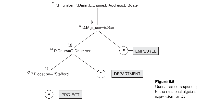
Note that the tree allows us to express the solution as a SEQUENCE of steps.
Another double-join example, listing employees and the projects they worked
on.
Select e.lname, p.pname from employee e,
works_on w, project p
where e.ssn = w.essn and w.pno = p.pnumber;