Normalization
Read in Elmasri & Navathe
- EN6 Chapter 15 / EN7 Chapter 14: Basics of Functional Dependencies and
Normalization for Relational Databases
- EN6 Chapter 16 / EN7 Chapter
15: Relational Database Design Algorithms and Further Dependencies
Normalization refers to a mathematical process for
decomposing tables into component tables; it is part of a broader area of
database design. The criteria that guide this are functional
dependencies, which should really be seen as user- and DBA-supplied
constraints on the data.
Our first design point will be to make sure that relation and entity
attributes have clear semantics. That is, we can easily explain attributes,
and they are all related. E&N spells this out as follows:
E&N
Guideline 1: Design a relation schema so that it is easy to explain its
meaning. Do not combine attributes from multiple entity types and
relationship types into a single relation.
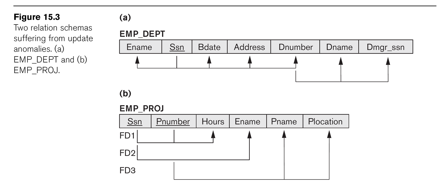
As examples, consider
EMP_DEPT
Ename
Ssn
Bdate
Address
Dnumber
Dname
Dmgr_ssn
create view emp_dept as select e.lname,
e.ssn, e.bdate, d.dnumber, d.dname, d.mgr_ssn
from employee e join department d on e.dno = d.dnumber;
This mixes employee information with department information.
Another example is
EMP_PROJ
Ssn
Pnumber
Hours
Ename
Pname
Plocation
create view emp_proj as select e.ssn,
p.pnumber, w.hours, e.lname, p.pname, p.plocation
from employee e, works_on w, project p where e.ssn=w.essn and w.pno =
p.pnumber;
Both these later records can lead to anomalies of the
following types:
- insertion anomalies: when
adding an employee, we must assign them to a department or else use
NULLs. When adding a new department with no employees, we have to use
NULLs for the employee Ssn, which is supposed to be the primary key!
- deletion anomalies: if we
delete the last EMP_DEP record from a department, we have lost the
department!
- update anomalies: what if we
update some EMP_DEPs with the new Dmgr_ssn, but not others?
This leads to
E&N
Guideline 2: design your database so there are no insertion, deletion,
or update anomalies. If this is not possible, document any anomalies
clearly so that the update software can take them into account.
The third guideline is about reducing NULLs, at least for frequently used
data. Consider the example of a disjoint set of inherited entity types,
implemented as a single fat entity table. Secretaries, Engineers, and
Managers each have their own attributes; every record has NULLs for two out
of these three.
E&N
Guideline 3: NULLs should be used only for exceptional conditions. If
there are many NULLs in a column, consider a separate table.
The fourth guideline is about joins that give back spurious tuples. Consider
EMP_LOCS
Ename
Plocation
EMP_PROJ1
Ssn
Pnumber
Hours
Pname
Plocation
If we join these two tables on field Plocation, we do not get what we want!
(We would if we made EMP_LOCS have
Ssn instead of Ename, and then joined the two on the Ssn column.) We can
create each of these as a view:
create view emp_locs as select e.lname,
p.plocation from employee e, works_on w, project p
where e.ssn=w.essn and w.pno=p.pnumber;
create view emp_proj1 as select e.ssn, p.pnumber, w.hours, p.pname,
p.plocation
from employee e, works_on w, project p where e.ssn=w.essn and w.pno =
p.pnumber;
Now let us join these on plocation:
select * from emp_locs el, emp_proj1
ep where el.plocation = ep.plocation;
Oops. What is wrong?
E&N
Guideline 4: Design relational schemas so that they can be joined with
equality conditions on attributes that are appropriatedly related
⟨primary key, foreign key⟩ pairs in a way that guarantees that no
spurious tuples are generated. Avoid relations that contain matching
attributes that are not ⟨foreign key, primary key⟩ combinations.
Problem: what do we have to do to meet the above guidelines?
Functional Dependencies and Normalization
A functional dependency is a kind of semantic
constraint. If X and Y are sets of attributes (column names) in a
relation, a functional dependency X⟶Y means that if two records have equal
values for X attributes, then they also have equal values for Y.
For example, if X is a set including the key
attributes, then X⟶{all attributes}.
Like key constraints, FD constraints are not based on specific sets of
records. For example, in the US, we have {zipcode}⟶{city}, but we no longer
have {zipcode}⟶{areacode}.
In the earlier EMP_DEPT we had FDs
Ssn ⟶ Ename, Bdate, Address, Dnumber
Dnumber ⟶ Dname, Dmgr_ssn
In EMP_PROJ, we had FDs
Ssn ⟶ Ename
Pnumber ⟶ Pname, Plocation
{Ssn, Pnumber} ⟶ Hours
Sometimes FDs are a problem, and we might think that just discreetly
removing them would be the best solution. But they often represent important
business rules; we can't really do that either. At the very least, if we
don't "normalize away" a dependency we run the risk that data can be entered
so as to make the dependency fail.
A superkey (or key
superset) of a relation schema is a set of attributes S so that no
two tuples of the relationship can have the same values on S. A key
is thus a minimal superkey: it is a
superkey with no extraneous attributes that can be removed. For example,
{Ssn, Dno} is a superkey for EMPLOYEE, but Dno doesn't matter (and in fact
contains no information relating to any other employee attributes); the key
is {Ssn}.
Note that, as with FDs, superkeys are related to the sematics of the
relationships, not to particular data in the tables.
Relations can have multiple keys, in which case each is called a candidate
key. For example, in table DEPARTMENT, both {dnumber} and {dname}
are candidate keys. For arbitrary performance-related reasons we designated
one of these the primary key; other
candidate keys are known as secondary keys.
(Most RDBMSs create an index for the primary key, but not
for other candidate keys unless requested.)
A prime attribute is an attribute
(ie column name) that belongs to some
candidate key. A nonprime attribute is not part of any key. For
DEPARTMENT, the prime attributes are dname and dnumber; the nonprime are
mgr_ssn and mgr_start.
A dependency X⟶A is full if the
dependency fails for every proper subset X' of X; the dependency is partial
if not, ie if there is a proper
subset X' of X such that X'⟶A. If A is the set of all attributes,
then the X⟶A dependency is full if X is a key, and is partial if X is a
non-minimal superkey.
Normal Forms and Normalization
Normal Forms are rules for well-behaved relations. Normalization is the
process of converting poorly behaved relations to better behaved ones.
First Normal Form
First Normal Form (1NF) means that a relation has no composite attributes or
multivalued attributes. Note that dealing with the multi-valued location
attribute of DEPARTMENT meant that we had to create a new table LOCATIONS.
Composite attributes were handled by making each of their components a
separate attribute.
Alternative ways for dealing with the multivalued location attribute would
be making ⟨dnumber, location⟩ the primary key, or supplying a fixed number
of location columns loc1, loc2, loc3, loc4. For the latter approach, we must
know in advance how many locations we will need; this method also introduces
NULL values.
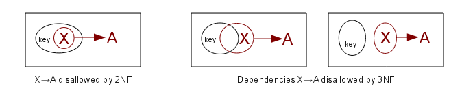
Second Normal Form
Second Normal Form (2NF) means that, if K represents the set of attributes
making up the primary key, every nonprime
attribute A (that is an attribute not a member of any key) is functionally
dependent on K (ie K⟶A), but that this fails for any proper subset of K (no
proper subset of K functionally determines A).
Note that if a relation has a single-attribute primary key, as does
EMP_DEPT, then 2NF is automatic. (Actually, the general definition of 2NF
requires this for every candidate key; a relation with a single-attribute
primary key but with some multiple-attribute other key would still have to
be checked for 2NF.)
We say that X⟶Y is a full
functional dependency if for every proper subset X' of X, X' does not
functionally determine Y. Thus, 2NF means that for every nonprime attribute
A, the dependency K⟶A is full: no
nonprime attribute depends on less than the full key.
In the earlier EMP_PROJ relationship, the primary key K is {Ssn, Pnumber}.
2NF fails because {Ssn}⟶Ename, and {Pnumber}⟶Pname, {Pnumber}⟶Plocation.
Table Factoring
Given a relation ⟨K1, K2, A1, A2⟩ and a functional dependency, eg
K1⟶A1, we can factor out the dependency into its own
relationship and a reduced version of the original relationship. The
original table has the righthand side of the dependency removed, and the new
table consists of both sides of the dependency. In this case, we get:
original: ⟨K1, K2, A2⟩ -- A1
removed
new: ⟨K1, A1⟩
-- both sides of
K1⟶A1
To put a table in 2NF, use factoring. If two new tables have a common full
dependency (key) on some subset K' of K, combine them. For EMP_PROJ, the
result of factoring is:
⟨Ssn, Pnumber, Hours⟩
⟨Ssn, Ename⟩
⟨Pnumber, Pname, Plocation⟩
Note that Hours is the only attribute with a full dependency on
{Ssn,Pnumber}.
The table EMP_DEPT is in 2NF, as is any table with a single key attribute.
Note that we might have a table ⟨K1, K2, K3, A1, A2, A3⟩, with dependencies
like these:
{K1,K2,K3}⟶A1 is full
{K1,K2}⟶A2 is full (neither K1 nor K2 alone determines
A2)
{K2,K3}⟶A2 is full
{K1,K3}⟶A3 is full
{K2,K3}⟶A3 is full
The decomposition could be this, if we factor on {K1,K2}⟶A2 and then
{K1,K3}⟶A3:
⟨K1, K2, K3, A1⟩
⟨K1, K2, A2⟩
⟨K1, K3, A3⟩
or it could be this, if we first
factor on {K2,K3}⟶A2 and then on {K2,K3}⟶A3.
⟨K1, K2, K3, A1⟩
⟨K2, K3, A2⟩
⟨K2, K3, A3⟩
The latter two can be coalesced into ⟨K2, K3, A2, A3⟩. However, there is no
way of continuing the first factorization approach and the second to find
some common final factorization. We do not have unique factorization!
Remember, dependency constraints can be arbitrary! Dependency constraints
are often best thought of as "externally imposed rules"; they come out of
the user-input-and-requirements phase of the DB process. Trying to pretend
that there is not a dependency constraint is sometimes a bad idea.
Consider the LOTS example of Fig 15.12.
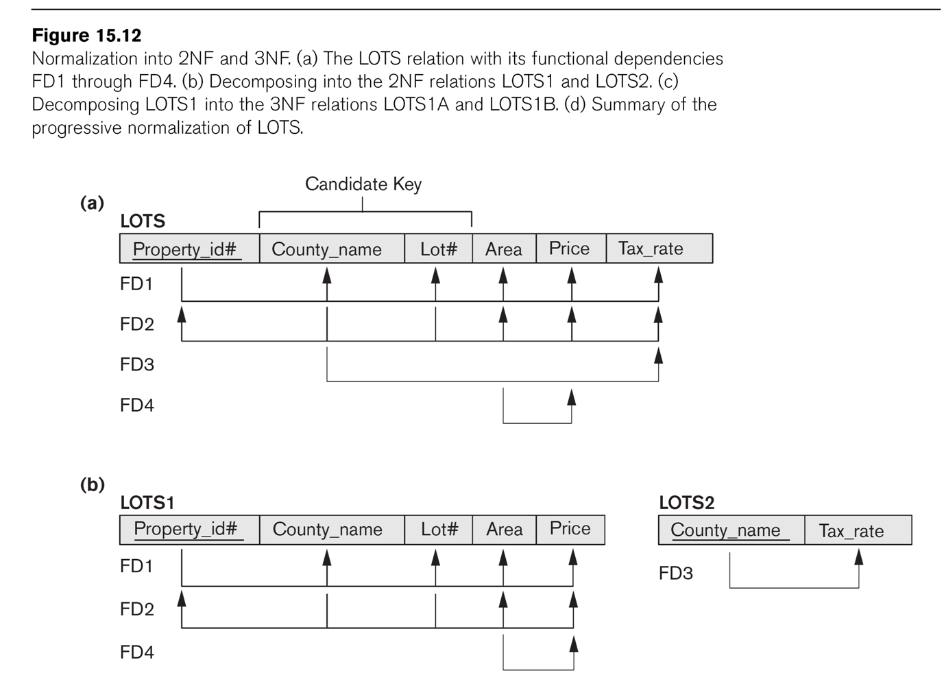
Attributes for LOTS are
- property_ID
- county
- lot_num
- area
- price
- tax_rate
The primary key is property_ID, and ⟨county,lot_num⟩ is also a key. These
are functional dependencies FD1 and FD2 respectively. We also have
FD3: county ⟶ tax_rate
FD4: area ⟶ price
(For farmland, FD4 is not completely unreasonable, at least if price refers
to the price for tax purposes. In Illinois, the formula is tax_price = area
× factor_determined_by_soil_type).
2NF fails because of the dependency county ⟶ tax_rate; FD4 does not violate
2NF. E&N suggest the decomposition into LOTS1(property_ID, county,
lot_num, area, price) and LOTS2(county, tax_rate).
We can algorithmically use a 2NF-violating FD to define a decomposition into
new tables. If X⟶A is the FD, we remove A from table R, and construct a new
table with attributes those of X plus A. E&N did this above for FD3:
county ⟶ tax_rate.
Before going further, perhaps two points should be made about decomposing
too far. The first is that all the functional dependencies should still
appear in the set of decomposed tables; the second is that reassembling the
decomposed tables with the "obvious" join should give us back the original
table, that is, the join should be lossless.
A lossless join means no information is lost, not that no records
are lost; typically, if the join is not lossless then we get back all the
original records and then some.
In Fig 15.5 there was a proposed decomposition into EMP_LOCS(ename,
plocation) and EMP_PROJ1(ssn,pnumber,hours,pname,plocation). The join was
not lossless.
Third Normal Form
Third Normal Form (3NF) means that the relation is in 2NF and also there is
no dependency X⟶A for nonprime attribute A and for attribute set X that does not contain a candidate key (ie X
is not a superkey). In other words, if X⟶A holds for some nonprime A, then X
must be a superkey. (For comparison, 2NF says that if X⟶A for nonprime A,
then X cannot be a proper subset of any key, but X can still overlap with a
key or be disjoint from a key.)
2NF: If K represents the set of attributes making up the primary key,
every nonprime attribute A (that is
an attribute not a member of any key) is functionally dependent on K (ie
K⟶A), but that this fails for any proper subset of K (no proper subset of K
functionally determines A).
3NF: 2NF + there is no dependency X⟶A for nonprime attribute A and for an
attribute set X that does not contain
a key (ie X is not a superkey).
Recall that a prime attribute is an
attribute that belongs to some key.
A nonprime attribute is not part of any key. The reason for the
nonprime-attribute restriction on 3NF is that if we do have a dependency
X⟶A, the general method for improving the situation is to "factor out" A
into another table, as below. This is fine if A is a nonprime attribute, but
if A is a prime attribute then we just demolished a key for the original
table! Thus, dependencies X⟶A involving a nonprime A are easy to fix; those
involving a prime A are harder.
If X is a proper subset of a key, then we've ruled out X⟶A for nonprime A in
the 2NF step. If X is a superkey,
then X⟶A is automatic for all A. The remaining case is where X may contain
some (but not all) key attributes, and also some nonkey attributes. An
example might be a relation with attributes K1, K2, A, and B, where K1,K2 is
the key. If we have a dependency K1,A⟶B, then this violates 3NF. A
dependency A⟶B would also violate 3NF.
3NF Table Factoring
Either case of a 3NF-violating dependency can be fixed by factoring out as
with 2NF: if X⟶A is a functional dependency, then to factor out this
dependency we remove column A from the original table, and create a new
table ⟨X,A⟩. For example, if the ⟨K1,
K2, A, B⟩ has 3NF-violating dependency K1,A⟶B, we create two new
tables ⟨K1, K2, A⟩ and ⟨K1, A, B⟩. If the dependency
were instead A⟶B, we would reduce the original table to ⟨K1,
K2, A⟩ and create new table ⟨A,B⟩.
Both the resultant tables are projections
of the original; in the second case, we also have to remove duplicates.
Note again that if A were a prime attribute, then it would be part of a key,
and factoring it out might break that key!
One question that comes up when we factor (for either 2NF
or 3NF) is whether it satisfies the nonadditive
join property (or lossless join
property): if we join the two resultant tables on the "factor"
column, are we guaranteed that we will recover the original table exactly?
The answer is yes, provided the factoring was based on FDs as above.
Consider the decomposition of R = ⟨K1,
K2, A, B⟩ above on the dependency K1,A⟶B into R1 = ⟨K1,
K2, A⟩ and R2 = ⟨K1, A,
B⟩, and then we form the join R1⋈R2 on the columns K1,A. If ⟨k1,k2,a,b⟩ is a
record in R, then ⟨k1,k2,b⟩ is in R1 and ⟨k1,a,b⟩ is in R2 and so
⟨k1,k2,a,b⟩ is in R1⋈R2; this is the easy direction and does not require any
hypotheses about constraints.
The harder question is making sure R1⋈R2 does not contain added
records. If ⟨k1,k2,a,b⟩ is in R1⋈R2, we know that it came from ⟨k1,k2,a⟩ in
R1 and ⟨k1,a,b⟩ in R2. Each of these partial records came from the
decomposition, so there must be b' so ⟨k1,k2,a,b'⟩ is in R, and there must
be k2' so ⟨k1,k2',a,b⟩ is in R, but in the most general case we need not
have b=b' or k2=k2'. Here we use the key
constraint, though: if ⟨k1,k2,a,b⟩ is in R, and ⟨k1,k2,a,b'⟩ is in
R, and k1,k2 is the key, then b=b'. Alternatively we could have used the dependency K1,A⟶B: if this dependency
holds, then it implies that if R contains ⟨k1,k2,a,b⟩ and ⟨k1,k2,a,b'⟩, then
b=b'.
This worked for either of two reasons: R1 contained the original key, and
R2's new key was the lefthand side of a functional dependency that held in
R.
In general, if we factor a relation R=⟨A,B,C⟩ into R1=⟨A,B⟩ and R2=⟨A,C⟩, by
projection, then the join R1⋈R2 on column A might be much larger
than the original R. As a simple example, consider Works_on =
⟨essn,pno,hours⟩; if we factor into ⟨essn,pno⟩ and ⟨pno,hours⟩ and then
rejoin, then essn,pno will no longer even be a key. Using two records of the
original data,
123456789
|
1
|
32.5
|
453453453
|
1
|
20
|
we see that the factored tables would contain ⟨123456789,1⟩ and ⟨1,20⟩, and
so the join would contain ⟨123456789,1,20⟩ violating the key constraint.
The relationship EMP_DEPT of EN fig 15.11 is not 3NF, because of the
dependency dnumber ⟶ dname (or dnumber ⟶ dmgr_ssn).
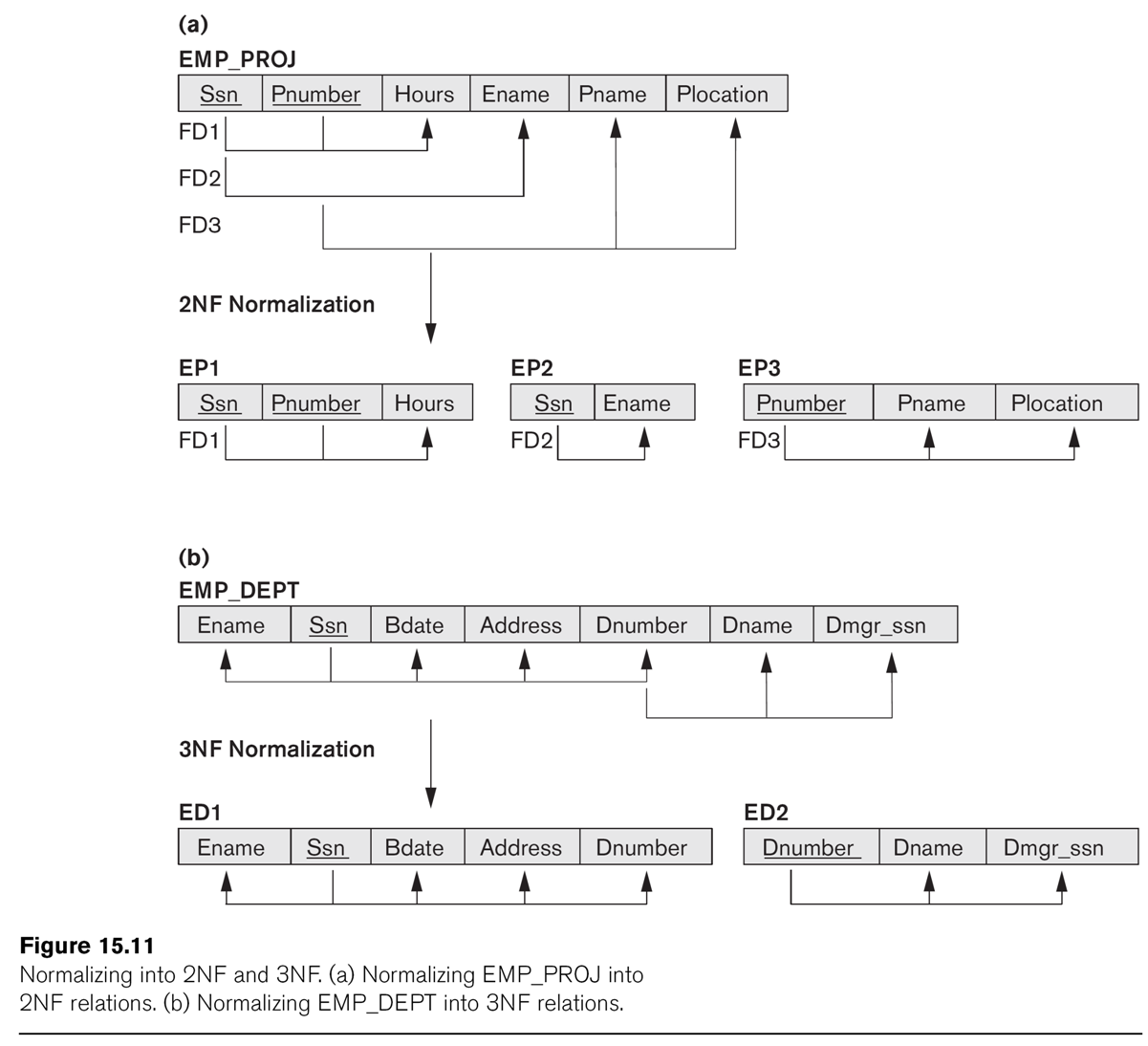
Can we factor this out?
The LOTS1 relation above (EN fig 15.12) is not 3NF, because of Area ⟶ Price.
So we factor on Area ⟶ Price, dividing into LOTS1A(property_ID,
county,lot_num,area) and LOTS1B(area,price). Another approach would be to
drop price entirely, if it is in fact proportional
to area, and simply treat it as a computed attribute.
4343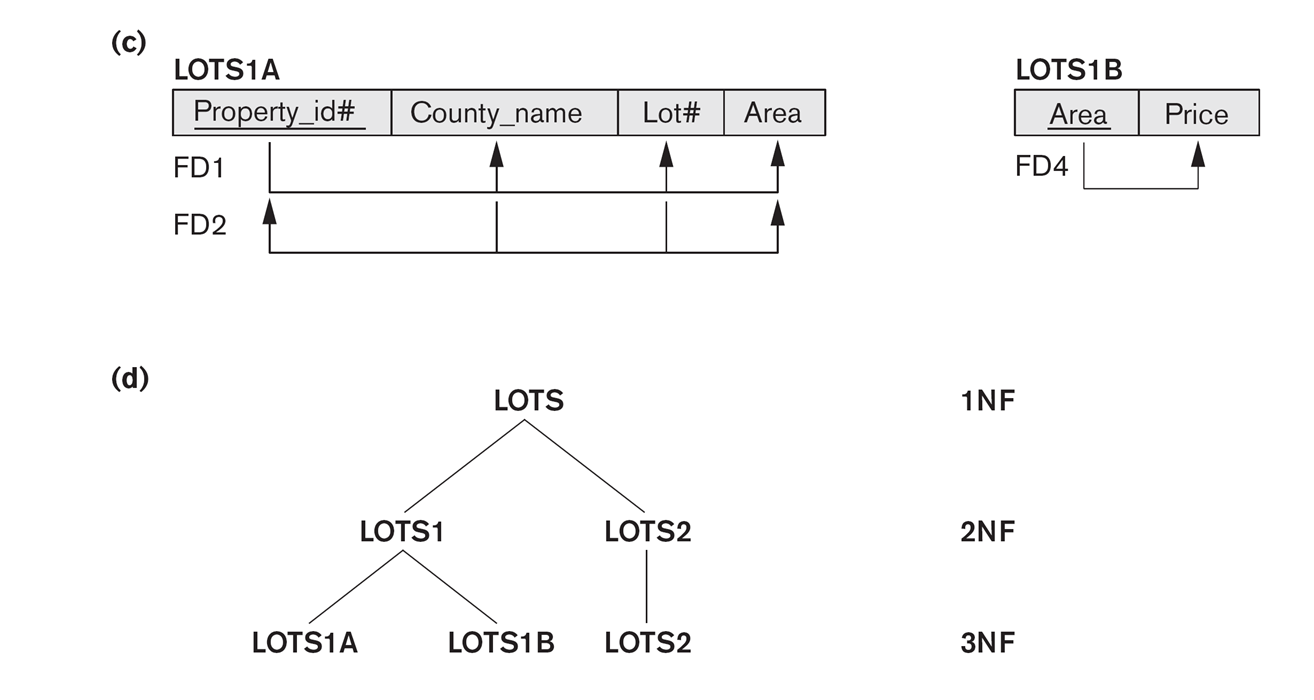
Multiple factoring outcomes
Consider a relation ⟨K1, K2, A, B, C⟩ where K1,K2 is the key and we have
dependencies K1⟶B and B⟶C. If we try to put into 2NF first,
by "factoring out" K1⟶B, we get tables ⟨K1,K2,A,C⟩ and ⟨K1,B⟩; the
dependency B⟶C is no longer expressible in terms of the tables. But if we
start by factoring out B⟶C, we get ⟨K1,K2,A,B⟩ and ⟨B,C⟩; we can now factor
out K1⟶B which yields relations ⟨K1,K2,A⟩, ⟨K1,B⟩ and ⟨B,C⟩; all functional
dependencies have now been transformed into key
constraints. Factoring can lose
dependencies, or, more accurately, make them no longer expressible except in
terms of the re-joined tables.
An aid to dealing with this sort of situation is to notice that in effect we
have a three-stage dependency: K1⟶B⟶C. These are often best addressed by
starting with the downstream (B⟶C) dependency.
Boyce-Codd Normal Form
BCNF requires that whenever there is a nontrivial functional dependency X⟶A,
then X is a superkey, even if A is a prime attribute. It differs from 3NF in
that 3NF requires either that X be
a superkey or that A be prime (a
member of some key). To put it another way, BCNF bans all nontrivial
nonsuperkey dependencies X⟶A; 3NF makes an exception if A is prime.
As for 3NF, we can use factoring to put a set of tables into BCNF. However,
there is now a serious problem: by factoring out a prime
attribute A, we can destroy an existing key constraint! To say this is
undesirable is putting it mildly.
The canonical "formal" example of a relation in 3NF but not BCNF is ⟨A,
B, C⟩ where we also have
C⟶B. Factoring as above leads to ⟨A, C⟩ and ⟨C, B⟩. We have lost the key A,B!
However, this isn't quite all it appears, because from C⟶B
we can conclude A,C⟶B, and thus that A,C is also a key, and might
be a better choice of key than A,B.
LOTS1A from above was 3NF and BCNF. But now let us suppose that DeKalb
county lots have sizes <= 1.0 acres, while Fulton county lots have sizes
>1.0 acres; this means we now have an
additional dependency FD5: area⟶county. This violates BCNF, but not
3NF as county is a prime attribute. (The second author Shamkant Navathe is
at Georgia Institute of Technology so we can assume DeKalb County is the one
in Georgia, not the one in Illinois, and hence is pronounced "deKAB".)
If we fix LOTS1A as in Fig 15.13, dividing into LOTS1AX(property_ID,area,lot_num)
and
LOTS1AY(area,county), then
we lose the functional dependency FD2:
(county,lot_num)⟶property_ID.
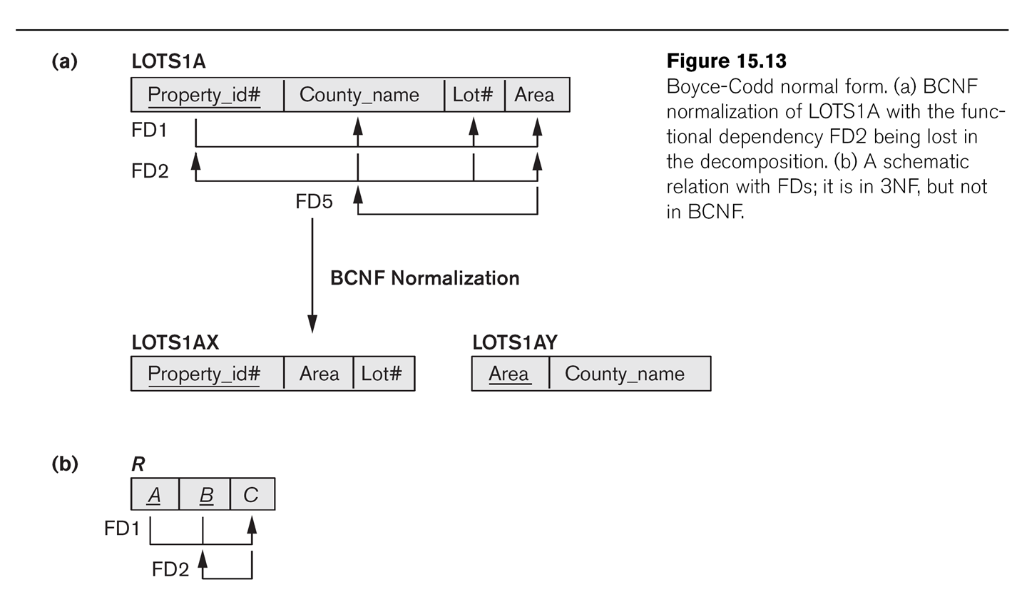
Where has it gone? This was more than just a random FD; it was a candidate key for LOTS1A.
All databases enforce primary-key constraints. One could use a CHECK
statement to enforce the lost FD2 statement, but this is often a lost cause.
CHECK (not exists (select ay.county,
ax.lot_num, ax.property_ID, ax2.property_ID
from LOTS1AX ax, LOTS1AX ax2, LOTS1AY ay
where ax.area = ay.area and ax2.area = ay.area
// join condition
and ax.lot_num = ax2.lot_num
and ax.property_ID <> ax2.property_ID))
We might be better off ignoring FD5 here, and just allowing for the
possibility that area does not determine county, or determines it only "by
accident".
Generally, it is good practice to normalize to 3NF, but it is often not
possible to achieve BCNF. Sometimes, in fact, 3NF is too inefficient, and we
re-consolidate for the sake of efficiency two tables factored apart in the
3NF process.
Fourth Normal Form
Suppose we have tables ⟨X,Y⟩ and ⟨X,Z⟩. If we join on X, we get ⟨X,Y,Z⟩. Now
choose a particular value of x, say x0, and consider all tuples ⟨x0,y,z⟩. If
we just look at the y,z part, we get a cross
product Y0×Z0, where Y0={y in Y | ⟨x0,y⟩ is in ⟨X,Y⟩} and
Z0={z in Z | ⟨x0,z⟩ is in ⟨X,Z⟩}. As an example, consider tables
EMP_DEPENDENTS = ⟨ename,depname⟩ and EMP_PROJECTS = ⟨ename,projname⟩:
EMP_DEPENDENTS
ename
|
depname
|
Smith
|
John
|
Smith
|
Anna
|
EMP_PROJECTS
ename
|
projname
|
Smith
|
projX
|
Smith
|
projY
|
Joining gives
ename
|
depname
|
projname
|
Smith
|
John
|
X
|
Smith
|
John
|
Y
|
Smith
|
Anna
|
X
|
Smith
|
Anna
|
Y
|
Fourth normal form attempts to recognize this in reverse, and undo it. The
point is that we have a table ⟨X,Y,Z⟩ (where X, Y, or Z may be a set
of attributes), and it turns out to be possible to decompose it into ⟨X,Y⟩
and ⟨X,Z⟩ so the join is lossless.
Furthermore, neither Y nor Z depend on X, as was the case with our 3NF/BCNF
decompositions.
Specifically, for the "cross product phenomenon" above to occur, we need to
know that if t1 = ⟨x,y1,z1⟩ and t2 = ⟨x,y2,z2⟩ are in ⟨X,Y,Z⟩, then so are
t3 = ⟨x,y1,z2⟩ and t4 = ⟨x,y2,z1⟩. (Note that this is the same condition as
in E&N, 15.6.1, p 533, but stated differently.)
If this is the case, then X is said to multidetermine
Y (and Z). More to the point, it means that if we decompose into ⟨X,Y⟩ and
⟨X,Z⟩ then the join will be lossless.
Are you really supposed even to look
for things like this? Probably not.
Fifth Normal Form
5NF is basically about noticing any other kind of lossless-join
decomposition, and decomposing. But noticing such examples is not easy.
16.4 and the problems of NULLs
"There is no fully satisfactory relational
design theory as yet that includes NULL values"
[When joining], "particular care must be
devoted to watching for potential NULL values in foreign keys"
Unless you have a clear reason for doing otherwise, don't let foreign-key
columns be NULL. Of course, we did just that in the EMPLOYEE table: we let
dno be null to allow for employees not yet assigned to a department. An
alternative would be to create a fictional department "unassigned", with
department number 0. However, we then have to assign Department 0 a manager,
and it has to be a real manager in
the EMPLOYEE table.
Denormalization
Sometimes, after careful normalization to produce an independent set of
tables, concerns about query performance lead to a regression to
less-completely normalized tables, in a process called denormalization. This
introduces the risk of inconsistent updates (like two records for the same
customer, but with different addresses), but maybe that's a manageable risk.
Maybe your front-end software can prevent this, and maybe it doesn't matter
that much.
As an example, suppose we have the following tables, with key fields
underlined. (Unlike the company database we are used to, projects here each
have their own managers.)
project: pnumber,
pname, mgr_ssn
employee: ssn,
name, job_title, dno
works_on: essn,
pid, hours
Now suppose management works mostly with the following view:
create view assign as
select e.ssn, p.pnumber, e.name, e.job_title, w.hours, p.pname, p.mgr_ssn,
s.name
from employee e, project p, works_on w, employee s
where e.ssn = works_on.essn and works_on.pid = project.pnumber and
p.mgr_ssn = s.ssn
That is a four-table join! Perhaps having a table assign
would be more efficient.
Similarly, our earlier invoice table was structured like
this:
invoice: invoicenum,
cust_id, date
invitem: invoicenum,
partnum, quantity, price
part: partnum,
description, list_price
customer: cust_id, cust_name, cust_phone, cust_addr
To retrieve a particular customer's invoice, we have to search three tables.
Suppose we adopt instead a "bigger" table for invoice:
invoice2: invoicenum,
cust_id, cust_name, cust_phone, date, part1num, part1desc, part1quan,
part2num, part2desc,part2quan, part3num,
part3desc,part3quan, part4num, part4desc,part4quan
That is, invoice2 contains partial information about the
customer, and also information about the first four items ordered. These
items will also appear in invitem, along with any
additional parts.
This means that most queries about the database can be displayed by
examining only a single table. If this is a web interface, there might be a
button users could click to "see full order", but the odds are it would
seldom be clicked, especially if users discovered that response was slow.
The important thing for the software developers is to make sure that the invoice2
and invitem and customer tables,
which now contain a good deal of redundant information, do not contain any
inconsistencies. That is, whenever the customer's information is updated,
then the invoice2 table needs to be updated too. A query
such as the following might help:
select i.invoicenum, i.cust_id, i.cust_name,
c.cust_name, i.cust_phone, c.cust_phone
from invoice2 i join customer c on i.cust_id = c.cust_id
where i.cust_name <> c.cust_name or i.cust_phone <>
c.cust_phone
We might even keep both invoice and invoice2,
with the former regarded as definitive and the latter as faster.
The value invoice2.cust_phone might be regarded as redundant, but it also
might be regarded as the phone current as of the time the order was
placed. Similarly, the invitem.price value can be different from the
part.list_price because invitem.price represents either the price as of the
date the order was placed or else a discounted price.
Denormalization can be regarded as a form of materialized view;
that is, the denormalized table actually exists somewhere, and is updated
(or reconstructed) whenever its base tables are updated. However, if we
create the denormalized table on our own, without a view, then we have more
control over how often the table gets updated. Perhaps the management assign
table above would only need to be updated once a day, for example.
Denormalization works best if all the original tables involved are too large
to be stored in memory; the cost of a join with a table small enough to fit
in memory is quite small. For this reason, the invoice2
example might be better than the assign example, for which
the tables are mostly "small".
Facebook makes significant use of denormalization at
times. One of their best-known examples is Timeline. See highscalability.com/blog/2012/1/23/facebook-timeline-brought-to-you-by-the-power-of-denormaliza.html,
and the actual FB blog on which that article was based: https://www.facebook.com/note.php?note_id=10150468255628920.
The basic issue is that the individual posts on your Timeline may be
scattered all over the place. In particular, many of the posts were
originally associated with other users, and they have either been shared
to your Timeline, or Facebook has decided to display them on your timeline
too (Facebook's "Multifeed Aggregator" makes decisions here). While all of
your direct posts (and replies) might be on the same disk
partition, that's not likely for posts that started on someone else's
Timeline, eg when Alice posts something to her page and also to
Bob and Charlie's pages. Here's the summary of the problem:
Before we began Timeline, our existing data
was highly normalized, which required many round trips to the databases.
Because of this, we relied on caching to keep everything fast. When data
wasn’t found in cache, it was unlikely to be clustered together on disk,
which led to lots of potentially slow, random disk IO. To support our
ranking model for Timeline, we would have had to keep the entire data set
in cache, including low-value data that wasn’t displayed.
After denormalization, the data is sorted by (user, time). Copies of
posts are made as necessary, so that most Timeline data for one user is on
one disk (or disk cluster). Fetching records just by (user) is quite fast.
When the same post is to be displayed on the timelines of two or more
users; the denormalization here means that we make as many copies of the
post as necessary. See also big_data.html#sharding.
Finally, this is an interesting blog post: kevin.burke.dev/kevin/red
[Reddit keeps] a Thing Table and a Data Table.
Everything in Reddit is a Thing: users, links, comments, subreddits,
awards, etc. Things keep common attributes like up/down votes, a type, and
creation date. The Data table has three columns: thing id, key, value.
There’s a row for every attribute. There’s a row for title, url, author,
spam votes, etc. When they add new features they didn’t have to worry
about the database anymore. They didn’t have to add new tables for new
things or worry about upgrades. Easier for development, deployment,
maintenance.
It works for them. YMMV.