Files and Indexes
References in Elmasri & Navathe (EN)
- EN6 Chapter 17 / EN7 Ch 16: disks
- EN6 Chapter 18 / EN7 Ch 17:
indexing
Disks
Hashing
Primary Indexes
Secondary Indexes
ISAM
B-Trees
Uber's Indexing Bottleneck
EN6 Ch 17 / EN7 Ch 16: basics of mechanical disks
Databases are often too big to fit everything into main memory, even today,
and traditional disks work differently from memory, particularly when
"random" access (as opposed to linear access, below) is involved. We here
assume disks are "mechanical", with rotating platters; solid-state disks
behave quite differently.
Disks are composed of blocks. At
the hardware level the basic unit of the sector
is typically 512 bytes, but the operating system clusters these together
into blocks of size 5K-10K. In the Elder Days applications would specify
their blocksize, but that is now very rare.
A disk looks to the OS like an array of blocks, and any block can be
accessed independently. To access a block, though, we must first move the
read head to the correct track (the
seek time) and then wait for the correct block to come
around under the head (rotational latency). Typical mean seek times are
~3-4ms (roughly proportional to how far the read head has to move, so seeks
of one track over are more like a tenth that). For rotational latency we
must wait on average one-half revolution; at 6000 rpm that is 5ms. 6000 rpm
is low nowadays, a reasonable value here is again 3-4 ms and so accessing a
random block can take 6-8ms.
It is these seek and rotational delays that slow down disk-based I/O.
Managing disk data structures is
all about arranging things so as to minimize the number of disk-block
fetches (and, to a lesser extent, minimizing the time spent on seeks). This
is a very different mind-set from managing in-memory data structures, where
all fetches are more-or-less equal, L2-cache performance notwithstanding.
Disk access completely dominates memory access and almost all CPU
operations.
When processing a file linearly, a
common technique is read-ahead, or
double-buffering. As the CPU begins to process block N, the IO subsystem
requests block N+1. Hopefully, by the time the CPU finishes block N, block
N+1 will be available. Reading ahead by more than 1 block is also possible
(and in fact is common). Unix-based systems commonly begin sequential
read-ahead by several blocks as soon as a sequential pattern is observed, eg
the system reads 3-4 blocks in succession.
When handling requests from multiple processes, disks usually do not
retrieve blocks in FIFO order. Instead, typically the elevator
algorithm is used: the disk arm works from the low-numbered track
upwards; at each track, it handles all requests received by that time for
blocks on that track. When there are no requests for higher-numbered tracks,
the head moves back down.
Records can take up a variable amount space in a block; this is annoying, as
it makes finding the kth record on the block more tedious. Still, once the
block is in memory, accessing all the records is quick. It is rare for
blocks to contain more than a hundred records.
BLOBs (binary large objects) are usually not stored within records; the
records instead include a (disk) pointer to the BLOB.
For a discussion of how all this changes when using solid-state disks
(SSDs), see queue.acm.org/detail.cfm?id=2874238.
File organizations
The simplest file is the heap file,
in which records are stored in order of addition. Insertion is efficient;
search takes linear time. Deletion is also slow, so that sometimes we just
mark space for deletion. This is actually a reasonable strategy if an index
is provided on the key field, though.
Postgres generally uses the heap organization. We can see the block number
and record position with the ctid attribute.
Another format is to keep the records ordered (sorted) by some field, the ordering field. This is not necessarily
a key; for example, we could keep file Employee ordered by Dno. If the
ordering field is a key, we call it the ordering
key. Ordered access is now fast, and search takes log(N) time
(where N is the length of the file in
blocks and we are counting only block accesses). This is the case
even without an index, though an index may improve on binary search only
modestly.
Note that the actual algorithm for block-oriented binary search is slightly
different from the classic array version: if we have blocks lo
and hi, and know that the desired
value X must, if present, lie between these two blocks, then we retrieve the
block approximately in between, mid.
We then check to see one of these cases:
- X < key of first record
on block mid
- X > key of last record on
block mid
- X is between the keys, inclusive, and so either the record is on
block mid or is not found
Note also that the order relation used to order the file need not actually
have any meaning terms of the application! For example, logically it makes
no sense to ask whose SSN is smaller. However, storing an employee file
ordered by SSN makes lookups by SSN much faster.
MySQL keeps records ordered by the primary key, sort of. The actual
organization is as a B-tree (below) on the primary key.
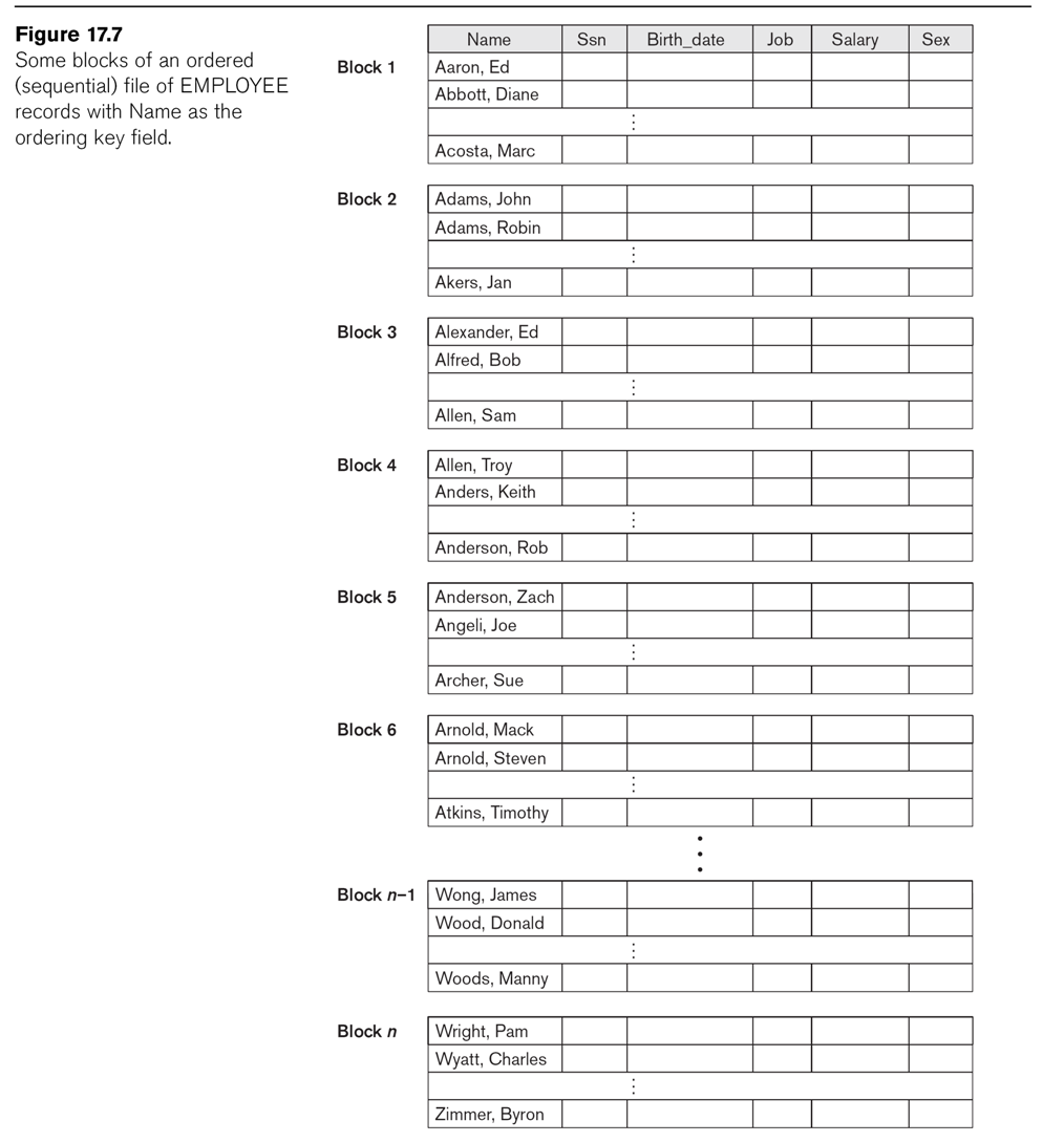
See Fig 17.7, in which a file uses ⟨lname, fname⟩ as its ordering fields.
The key is ssn; the file is not, however, ordered by ssn.
Insertion and deletion in ordered files expensive. We can improve insertion
by keeping some unused space at the end of each block for new records (or
the moved-back other records of the block). We can improve deletion by
leaving space at the end (or, sometimes, right in the middle).
Another approach is to maintain a transaction
file: a sequential file consisting of all additions and deletions.
Periodically we update the master file with all the transactions, in one
pass.
Multiple attributes
We can also, in principle, keep a file ordered by two attributes,
ordered lexicographically so (a,b) < (c,d) if a<c or (a=c and b<d).
The file in diagram 17.7 above is ordered by ⟨lname,fname⟩, but a file can
just as easily be ordered by two unrelated fields. Consider the works_on
file; we can regard it as ordered as follows:
| essn |
pno |
hours |
| 123456789 |
1 |
32.5 |
| 123456789 |
2 |
7.5 |
| 333445555 |
2 |
10 |
| 333445555 |
3 |
10 |
| 333445555 |
10 |
10 |
| 333445555 |
20 |
10 |
| 453453453 |
1 |
20 |
| 453453453 |
2 |
20 |
| 666884444 |
3 |
40 |
| 888665555 |
20 |
0 |
| 987654321 |
20 |
15 |
| 987654321 |
30 |
20 |
| 987987987 |
10 |
35 |
| 987987987 |
30 |
5 |
| 999887777 |
10 |
10 |
| 999887777 |
30 |
30 |
Records here are sorted on ⟨essn,pno⟩.
Hashing
Review of internal
(main-memory-based) hashing. We have a hash function h that applies to the
key values, h = hash(key).
- bucket hashing: the hash table component hashtable[h] contains a
pointer to a linked list of records for which hash(key) = h.
- chain hashing: if object Z hashes to value h, we try to put Z at
hashtable[h]. If that's full, we try hashtable[h+1], etc.
For disk files, we typically use full blocks as buckets. However, these will
often be larger than needed. As a result, it pays to consider hash functions
that do not generate too many different values; a common approach is to
consider hash(key) mod N, for a smallish N (sometimes though not universally
a prime number).
Given a record, we will compute h = hash(key). We also provide a
single-block map ⟨hash,block⟩ of hash values to block addresses (in effect
corresponding to hashtable[]). Fig 17.9 (not shown here) shows the basic
strategy: the hash function returns a bucket number, given a record, and the
hash table is a map from bucket numbers to disk-block addresses.
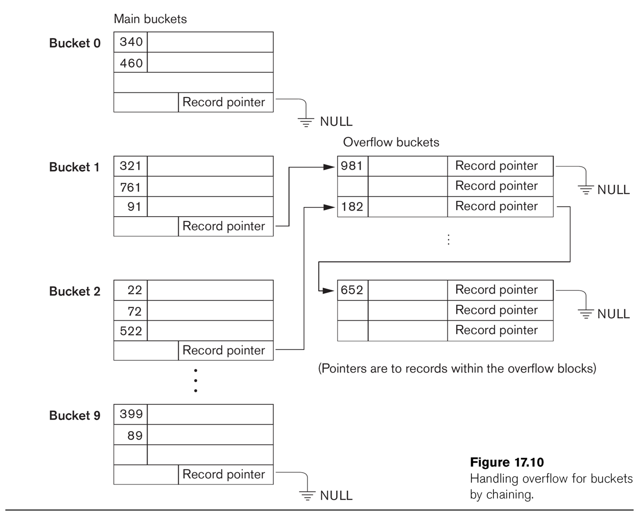
More detail on the buckets is provided in Fig 17.10, below, which also shows
some overflow buckets. Note that Bucket 1 and Bucket 2 share
an overflow bucket; we also can (and do) manipulate the ⟨hash,block⟩
structure so that two buckets share a block (by entering ⟨hash1,block1⟩ and
⟨hash2,block2⟩ where block1 = block2). When a single bucket approaches two
blocks, it can be given its own overflow block.
When more than one bucket shares an overflow bucket, it is likely we will
keep some expansion space between the two sets of records.
In this diagram, the hash function returns the last digit of the
key-field value (eg hash(127) = 7).
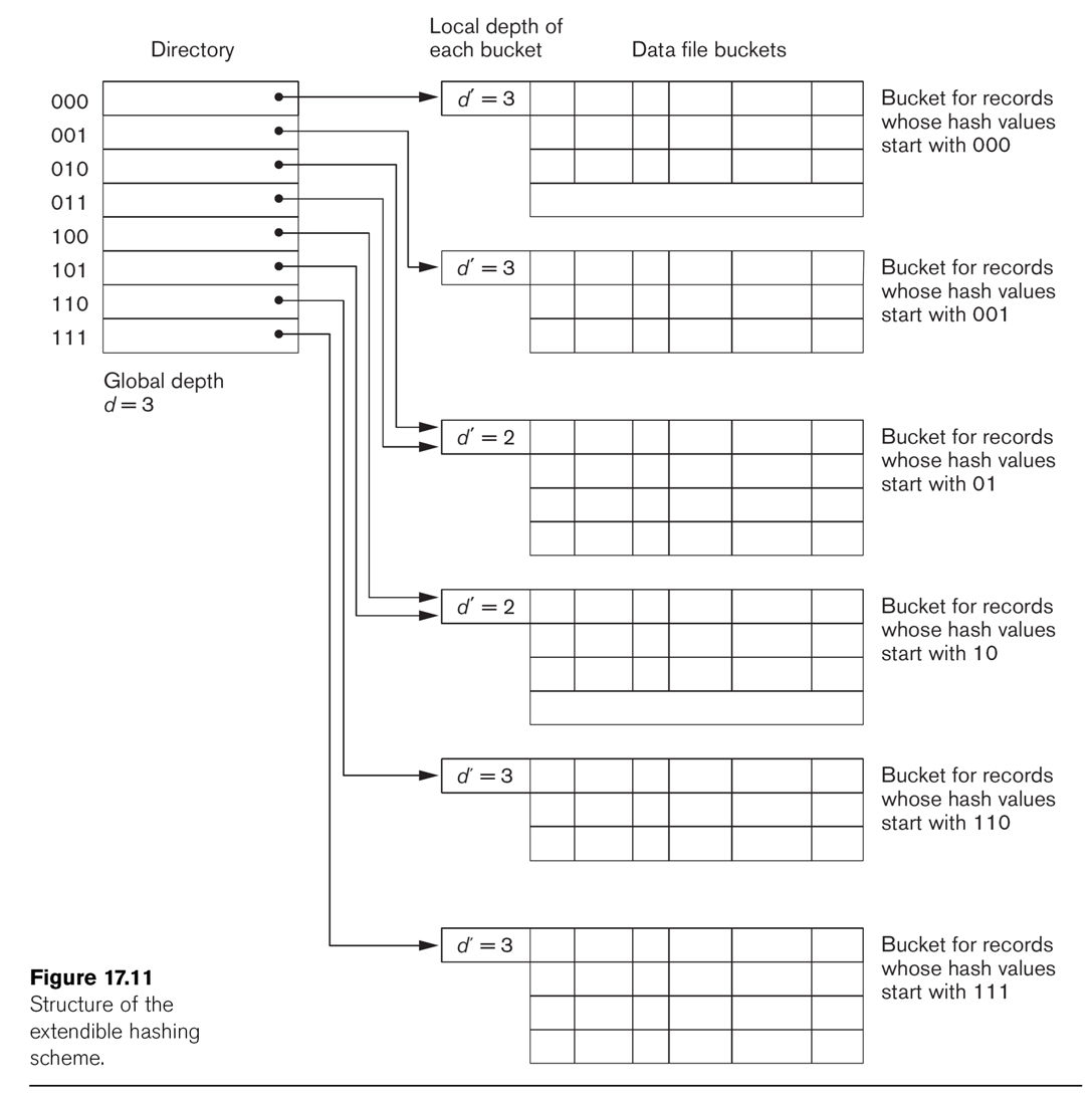
Extendible Hashing
This technique manages buckets more efficiently. We hash on the first d bits of the hash values; d is called
the global depth. We keep a
directory of all 2d possible values for these d bits, each with a
pointer to a bucket block. Sometimes, two neighboring buckets are consolidated
in the directory; for example, if d=3, hash prefix values 010 and 011 might
point to the same block. That block thus has a reduced local
depth of 2.
As we fill blocks, we need to create new ones. If a block with a reduced
local depth overflows, we split it into two blocks with a greater depth
(still ≤ d). If a block with local depth d overflows, we need to make some
global changes: we increment d by 1, double the directory size, and double
up all existing blocks except for the one causing the overflow.
For this to work well, it is helpful to have a hash function that
is as "pseudorandom" as possible, so for any prefix-length d the 2d
buckets are all roughly the same size. (The size inequality can be pretty
rough; even with perfect randomness the bucket sizes will be distributed
according to the Poisson distribution).
See Fig 17.11.
Extendible hashing grew out of dynamic
hashing, in which we keep a tree structure of hashcode bits,
stopping when we have few enough values that they will all fit into one
block.
EN6 Ch 18 / EN7 Ch 17: Indexing
It is near-universal for databases to provide indexes
for tables. Indexes provide a way, given a value for the indexed field, to
find the record or records with that field value. An index can be on either
a key field or a non-key field.
Indexes also usually provide a way to traverse the table,
by traversing the index. Even hash-based indexes usually support traversal,
though not in any "sensible" order. (That said, traversing a file in
increasing order of SSNs is not a logically meaningful operation either.)
If the file organization is such that records with the same index value are
found on the same or nearby blocks -- eg if the file is physically
ordered by the index field -- then the index is said to be clustered.
The records corresponding to the indexed field are all together.
An index can be sparse, meaning that there is not an
index entry for every record of the file. There is
typically an index entry for the first record of each block. If names are
a key field, and there are index entries for Alice (start of block 1) and
Charlie (start of block 2), then to find Bob one reasons that Bob <
Charlie so Bob has to be in block 1. The file has to be clustered for this
to work.
An index on a non-key field is considered sparse, if each value is
present in the index but the index entry for a value points to the set of
records having that value. This would include most if not all non-key
indexes.
The alternative to a sparse index is dense. Most
Postgres indexes are dense.
Primary Index
A primary index is a clustered
index on the primary key of a sorted
file. (Note that an index on the primary key, if the file is not maintained
as sorted on that primary key, is thus not
a "primary index"!)
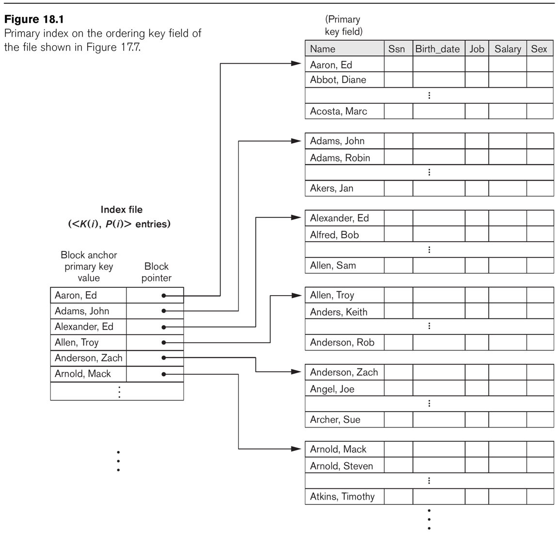
The index logically consists of an ordered list of pairs ⟨k,p⟩, where k is
the first key value to appear in the block pointed to by p (this first
record of each block is sometimes called the anchor
record). To find a value k in the file, we find consecutive ⟨k1,p⟩
and ⟨k2,p+1⟩ where k1≤k<k2; in that case, the record with key k must be
on block p. This is an example of a sparse
index: not every key value must appear in the index. A primary
index is usually much smaller than the file itself. See Fig
18.1.
The essential point here is that because the file is sorted by the key
value, the index needs many fewer entries than it otherwise would.
In MySQL 5.7, with the InnoDB engine, the primary-key index is a B-tree
and the entire records are kept as leaf nodes, in effect sorted by the key
value. This makes this kind of index a "primary index". For Postgres, an
index-clustered file structure is optional. If we issue the command
cluster tablename using indexname
then the table will be re-organized in clustered format. However,
additional insertions will not follow the clustering, so this is most
commonly done only on tables that are not actively written to.
Example 1 (from EN6 p 635) Suppose a file has 30,000 records, 10 per block,
for 3000 blocks. Direct binary search takes 12 block accesses. The index
entries have 9 bytes of data plus a 6-byte block pointer, for a total of 15
bytes, so 1024/15 = 68 index entries fit per 1024-byte block. The index
therefore has 3000/68 = 45 blocks; binary search requires 6 block accesses,
plus one more for the actual data block itself. There is also an excellent
chance that the entire 45-block index will fit in RAM.
Clustering of a primary index is useful only if we are traversing the table
in order, using the index. If we've looked up 'Adams', we know 'Aesop',
'Aftar' and 'Agatha' will be near by, possibly in the same block. E&N,
in fact, doesn't use the term "clustered" for such an index.
Non-key Clustering Index
If the index is on a non-key field, then one index entry
may correspond to multiple records. If the file is also ordered
on this nonkey field (think Employee.dno, or possibly Employee.lname), we
call it a clustering index. A file
can have only one clustering index, including primary indexes in this
category.
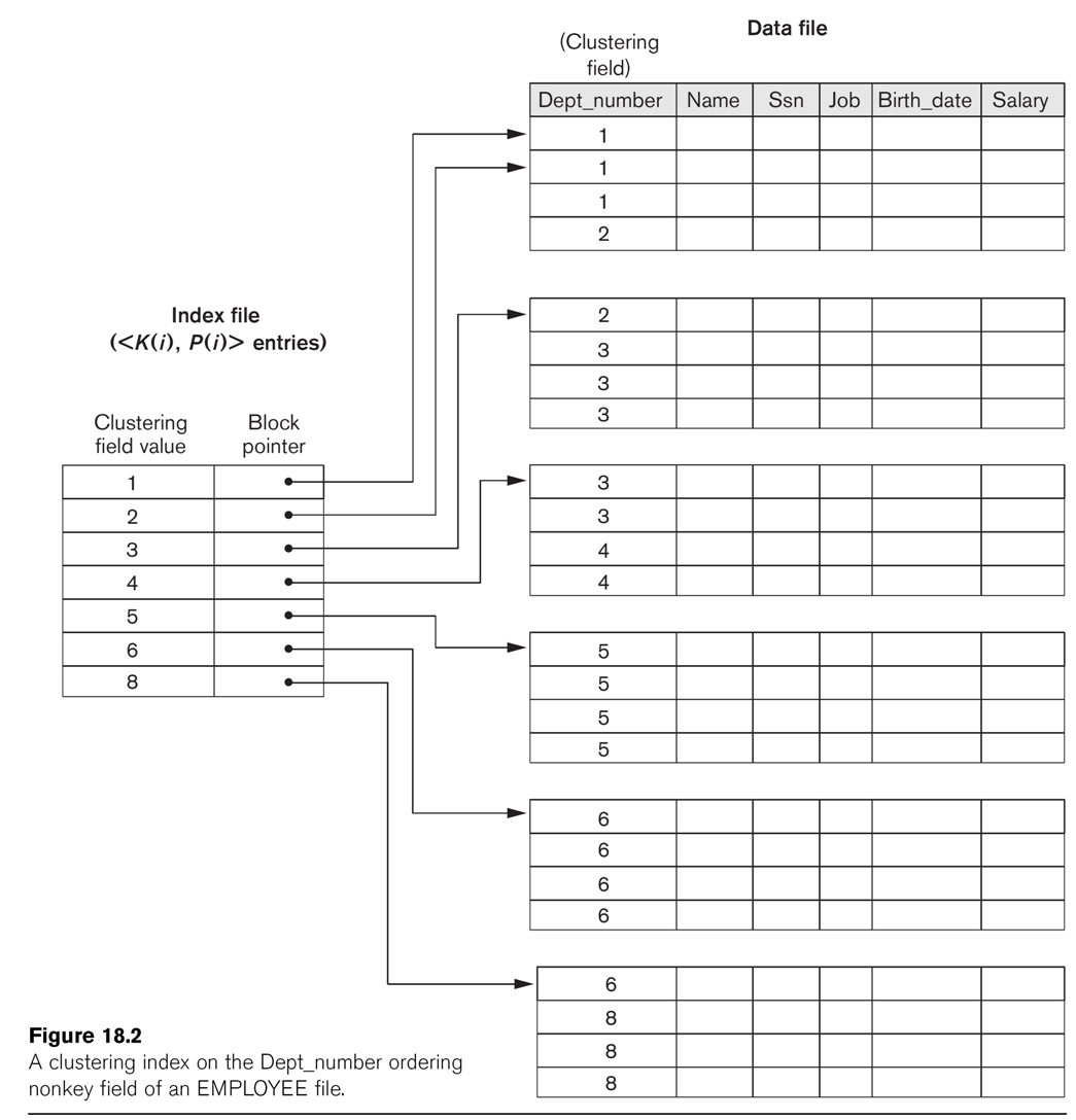
The index structure of a non-key clustering index is the same as before,
except now the block pointer points to the first block that contains any
records with that value; see Fig 18.2.
Such an index may or may not be sparse. In the example of Fig 18.2 the index
is dense: every dept_number value is included. In principle, we only need to
include in the index the attribute values that appear first in each block;
that is, dept_numbers 1, 2, 3, 5 and 6. But there is a tradeoff; if we skip
some index values then we likely will want an index entry for every block
(that is, for dept_number 6 there should be two blocks listed). For a
non-key index this may mean many more entries than an index entry for every
distinct value. In Fig 18.2, we have an entry for every distinct
value; we could remove the entries for Dept_number=2 and Dept_number=4.
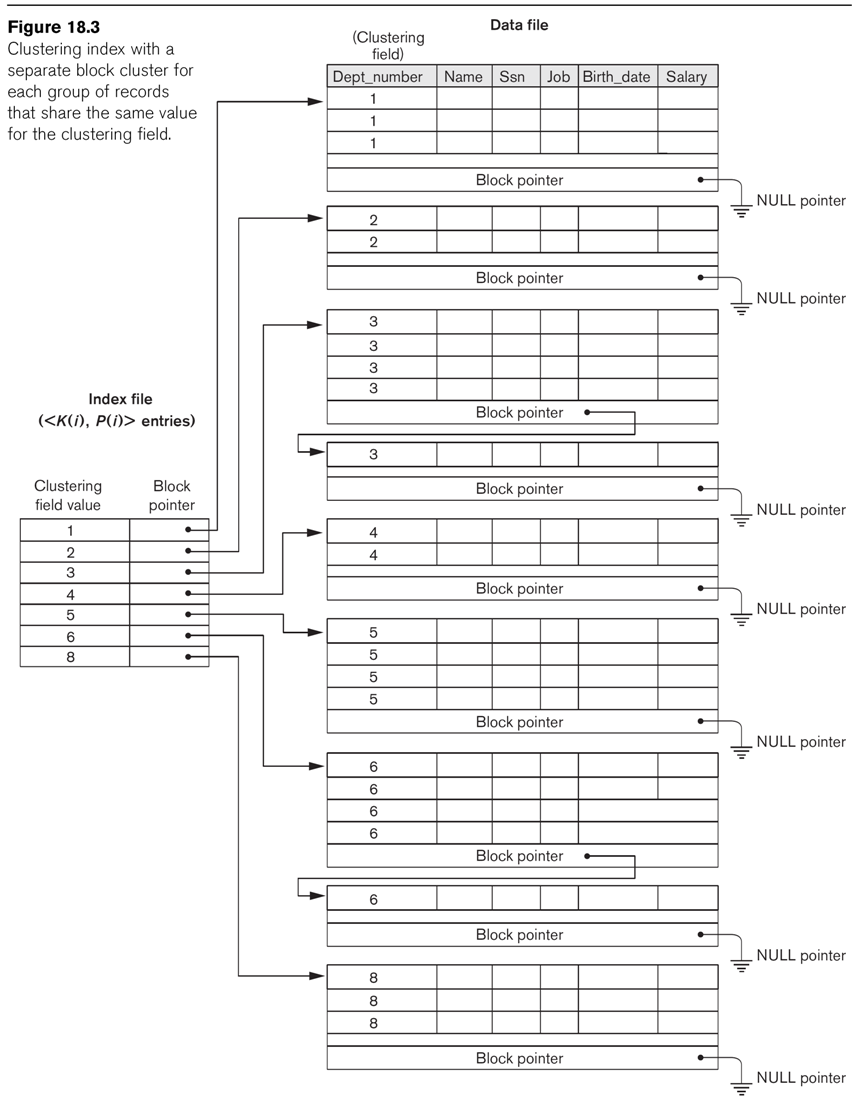
Another approach to clustering indexes may be seen in Fig
18.3, in which blocks do not contain records with different cluster
values. Note that this is again a method of organizing the file
for the purpose of the index.
Ordering a file by a non-key field may sound unlikely. However, it may be
quite useful in cases where the file has a multi-attribute key. For example,
we might keep the works_on file ordered by essn; the essn alone is not a
key. This would allow easy lookup of any employee's projects. We might in
fact keep the file ordered lexicographically by the full key, ⟨essn,pno⟩, in
which case the file would be automatically ordered by essn alone,
and we could create a clustering index on essn alone. Yet another example of
a plausible clustering index is the invoice_item file we considered
previously. The key is ⟨invoice_num, partnum⟩. Keeping the file ordered
first by invoice_num and second by partnum would allow a clustering index on
invoice_num alone, which is likely to be something we frequently need to do.
(This example is in some sense the same as the works_on example.)
A file can have multiple indexes, but the file itself can be structured
(clustered) for only one index. We'll start with that case. The simplest
file structuring for the purpose of indexing is simply to keep the file
sorted on the attribute being indexed; this allows binary search. For a
while, we will also keep restrict attention to single-level
indexes.
Secondary Indexes
Now suppose we want to create an index for Employee by (fname, lname),
assumed for the moment to be a secondary key.
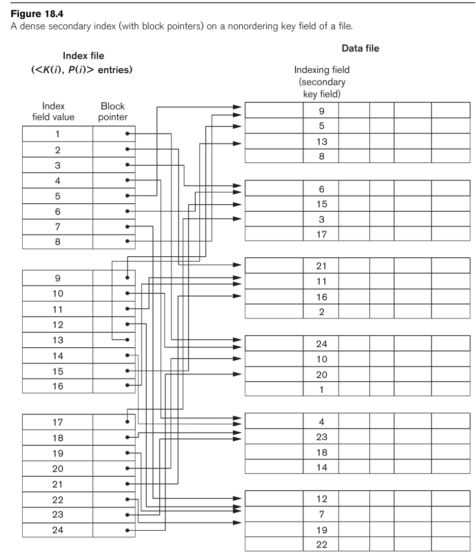
The record file itself is ordered by SSN, which is the primary key. An index
on a secondary key will necessarily
be dense, as the file won't be ordered by the secondary key; we cannot use
block anchors. A common arrangement is simply to have the index list
⟨key,block⟩ pairs for every key value appearing; if there are N records in
the file then there will be N in the index and the only savings is that the
index records are smaller. See Fig 18.4.
If B is the number of blocks in the original file, and BI is the number of
blocks in the index, then BI ≤B, but not by much, and log(BI) ≃ log(B), the
search time. But note that unindexed search is linear
now, because the file is not ordered on the secondary key.
Many MySQL indexes are of this type.
Example 2, EN6, p 640: 30,000 records, 10 per block. Without an index,
searching takes 3,000/2 = 1500 blocks on average. Blocks in the index hold
68 records, as before, so the index needs 30,000/68 = 442 blocks; log2(442)
≃ 9.
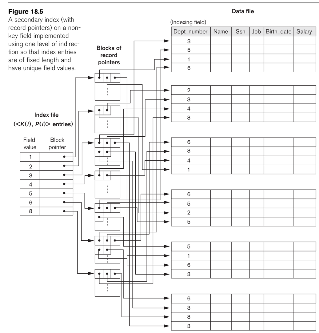
Secondary indexes can also be created on nonkey
fields. We can create dense indexes as above, but now with multiple entries
for the indexed attribute, one for each record (Option 1 in EN6 p 640). A
second approach (option 2 in EN6 p 640) is to have the index consist of a
single entry for each value of the indexed attribute, followed by a list
of record pointers. The third option, perhaps the most common, is for each
index entry to point to blocks of
record pointers, as in Fig 18.5.
| index on |
file ordered by |
|
|
example |
key value
(primary index) |
that key value |
sparse |
|
fig 18.1 |
key value
(secondary key?) |
something else |
dense |
|
fig 18.4 |
nonkey value
(clustering) |
that nonkey value |
sparse |
|
figs 18.2, 18.3 |
nonkey value
(clustering) |
something else |
sparse |
|
fig 18.5 |
Hashing Indexes
Hashing can be used to create a form of index, even if we do not structure
the file that way. Fig 18.15 illustrates
an example; the hash function in this example is the final digit of the sum
of the digits of the employee number.
Hashing with equality comparisons, but not order comparisons, which is to
say hashing can help us find a record with ssn=123456789, but not records
with salary between 40000 and 50000. Hash indexes are, in theory, a good
index for joins. Consider the join
select e.lname, w.pno, w.hours from employee e, works_on
w where e.ssn = w.essn;
We might choose each record e from employee, and want to find all records in
works_on with e.ssn = w.essn. A hash index for works_on, on the field essn,
can be useful here. Note this can work even though works_on.essn is not a
key field.
There is one problem: we are likely to be retrieving blocks of works_on in
semi-random order, which means one disk access for each record. However,
this is still faster than some alternatives.
MySQL supports adaptive hash indexes, which are related to
extendible hashing. Hash indexes are built on top of B-tree indexes, using
an empirically determined prefix of the B-tree key.
Sometimes the index is rebuilt with a longer prefix; this is the "adaptive"
part. Hash indexes are faster than B-tree indexes, but only work for
equality comparisons (including inner-query checks with IN), not ordering,
range or prefix comparisons. See https://dev.mysql.com/doc/refman/5.7/en/index-btree-hash.html.
Multilevel indexes & ISAM
Perhaps our primary sorted index grows so large that we'd like an index for
it. At that point we're creating a
multi-level index. To create this kind of index, we start with the primary
index, with an index entry for the anchor record of each block, or a
secondary index, with an entry for each record. Call this the base
level, or first level, of
the index. We now create a second level
index containing an index entry for the anchor record of each block of the
first-level index. See Fig 18.6. We keep
adding levels until we get to a top-level index that fits in a single block.
This is called an indexed sequential file,
or an ISAM (Indexed Sequential
Access Method) file.
This technique works as well on secondary keys, except that the first
level is now much larger.
MySQL has the MyISAM storage engine. This is no longer the default (having
been replaced by InnoDB, which supports foreign-key constraints), but MyISAM
is still a contender for high-performance read-heavy scenarios. (Because
MyISAM supports only table-level locking, rather than
InnoDB's row-level locking, write performance can
be a bottleneck, though MyISAM does support simultaneous record insertions.)
What is involved in inserting new
records into an ISAM structure? The first-level index has to be "pushed
down"; unless we have left space ahead of time, most blocks will need to be
restructured. Then the second and higher-level indexes will also need to be
rebuilt, as anchor records have changed.
Example: we have two records per block, and the first level is
Data file:
1 2 3
5 7 9 20
1st-level index: 1
3 7 20
2nd-level index: 1 7
What happens when we insert 8? 4? 6?
What happens when we "push up a level", that is, add an entry that forces us
to have one higher level of index?
EN6 Example 3 (p 644): 30,000 records and can fit 68 index entries per
block. The first-level index is 30,000/68 = 442 blocks, second-level index
is 442/68 = 7 blocks; third-level index is 1 block.
B-trees (Bayer trees)
Rudolf Bayer introduced these in a 1972 paper with Edward McCreight. The
meaning of the B was left unspecified, but they were in a sense
diametrically opposite to binary trees. In 2013 McCreight said the
following:
Bayer and I were in a lunchtime where we get
to think [of] a name. And ... B is, you know ... We were working for
Boeing at the time, we couldn't use the name without talking to lawyers.
So, there is a B. [The B-tree] has to do with balance, another B. Bayer
was the senior author, who [was] several years older than I am and had
many more publications than I did. So there is another B. And so, at the
lunch table we never did resolve whether there was one of those that made
more sense than the rest. What really lives to say is: the more you think
about what the B in B-trees means, the better you understand B-trees.
Consider a binary search tree for the moment. We decide which
of the two leaf nodes to pursue at each point based on comparison.
5
/ \
3 7
/ \ / \
2 4 6 8
We can just as easily build N-ary search trees, with N leaf nodes and N-1
values stored in the node. An ordered search tree might, for example, be ternary. However, we might just as
easily have a different N at each node!
50 80
/ |
\
20 40 60 90
100 120 150
/ | \
/ | |
\ \
2 30
45 85 95
110 130 151 155
Bayer trees are a form of N-ary search tree in which all the leaf nodes are
at the same depth. In this sense, the tree is balanced. As an example, let's
suppose we have a maximum of 4 data items per node. Here is a tree with a
single value in its root node and two (four-value_ leaf nodes:
15
/
\
1 4 8
9 20 22
25 28
Here's a tree with two values in its root node, and three leaf nodes. One of
the leaf nodes is not "full". (This tree cannot be reached by inserting
values into the tree above.)
15 30
/ | \
/
| \
1 4 8 9 20 22 25
28 31 37 42
How can we add nodes so as to remain balanced?
We also want to minimize partial blocks.
A B-tree of degree d
means that each block has at most d
tree pointers, and d-1 key
values. In addition, all but the top node has at least
(d-1)/2 key values. Generally we
want the order to be odd, so (d-1)/2 is a whole number. Many authors refer
to (d-1)/2 as the order p of the tree, though some don't,
and "degree" is standard everywhere.
To insert a value, you start at the root node and work down to the leaf
node that the new value should be inserted into. The catch is that the
leaf node may already have d-1 values, and be unable to accept one more.
B-trees deal with this using the "push-up" algorithm: to
add a new value to a full block, we split
the block and push up the median value to the parent block. (Conceptually,
in finding the median we add the newly inserted value temporarily. The
newly inserted value may end up being the median, but probably
won't.) After splitting, this leaves two sibling blocks (where there had
been one), each of size p = (d-1)/2, and one new value added to the parent
block (thus allowing one more child block, which we just created).
The parent block may now also have to be split. This process continues
upwards as long as necessary.
The tree only grows in height when the push-up process bumps up a new root
block; the tree remains balanced.
The parent block can have just one data value, but all the other blocks
are, at a minimum, half full; that is, the smallest a non-root block can
be is (d-1)/2.
Red-black trees are binary trees that are closely related to Bayer trees
of degree 4. Note that d=4 is odd, so such trees don't have a well-defined
order, and after splitting we end up with one block of size 1 and another
of size 2.
There is a java-applet animation of B-tree insertion at http://slady.net/java/bt/view.php?w=800&h=600.
It's getting old, and Java applets are riskier and riskier; another
animation is available at https://www.cs.usfca.edu/~galles/visualization/BTree.html.
B+ trees: slight technical improvement where we replicate all the key values
on the bottom level.
Indexes on multiple attributes
What about the works_on table with its index on (essn, pno) (or, for that
matter, (pno, essn))? Here the primary key involves two attributes.
Alternatively, perhaps we want an index on (lname, fname), even though it is
not a primary key.
We create an ordered index on two (or more) attributes by using the
lexicographic ordering: (a1,b1) comes before (a2,b2) if a1<a2 or
(a1=a2 and b1<b2). Such an ordered index can be sparse. If the
file is kept ordered this way, we can create a (sparse) primary index just
as for a single attribute: the index consists of pairs (a,b) of the anchor
record on each block. We can zip through the index looking for (a',b') until
we find an entry (a,b) that is too far: a>a' or else a=a' and b>b'. We
then know the value we're looking for, if present, will be found on the
previous block.
Example query (E&N6, p 660):
select e.fname, e.lname from employee e where e.dno = 4
and e.age=59;
If we have an index on dno, then access that cluster using the index and
search for age.
If we have an index on age, we can use that.
If we have an index on both attributes individually, we can get the block
numbers for each separate lookup and then take the intersection;
these are the only blocks we have to retrieve.
Alternatively, perhaps we have an index on (dno, age), in which case we have
a single lookup! But we also have expensive indexes to maintain. Generally
multi-attribute indexes are useful only when there is a multi-attribute key
or when lookup by both attributes is very frequent (as might be the case for
an index on (lname, fname)). In other words, a joint index on (dno,age) is
unlikely to be worth it.
It is also common to take an ordered index of (a,b) pairs and use it as a clustered
index on just the 'a' values; the original index is, after all, ordered by
the 'a' values. This allows rapid lookup based on either an (a) or an (a,b)
search key. For many index types, the original (a,b) index can be used as an
index on (a) alone.
Indexes on Prefixes
When an attribute is long, it is not uncommon to create an index on a prefix
of the key (instead of the entire key), at least if a prefix length can be
determined that is "almost as unique" as the attribute in question. For
example, we could create an index on the first 4 characters of employee.ssn,
if we thought it was unlikely many employees shared the same first four
digits in their SSNs. If the index was on employee.lname, we might create
the index on just the first 6 or 8 characters. Fixed-length comparisons tend
to be faster.
For Postgres, indexes will make use of string prefixes only if the index was
created with the text_pattern_ops
or varchar_pattern_ops
attribute (example: the password database).
Indexes v File Organization
What's the difference between creating a hashed file organization and a
hashed index? Or a B-tree file organization versus a B-tree index? An index
needs to stand alone, and allow finding any given record; a
file-organization method generally allows us to retrieve blocks
of records at a time.
A B-tree index technically has to be a B+-tree, as a B-tree includes file
blocks at interior levels. The usual B/B+ tree also includes many related
records in single leaf blocks, but that is straightforward to give up (at
the cost of less efficient traversal).
Uber and secondary indexes
In July 2016, Uber published a blog post about why they were switching from
Postgres to MySQL: eng.uber.com/mysql-migration.
At least one of their performance bottlenecks was apparently the need to
constantly update the location of every driver and user. To do this, they
needed on the order of a million writes a second; see highscalability.com/blog/2016/9/28/how-uber-manages-a-million-writes-per-second-using-mesos-and.html.
The million-writes-per-second issue doesn't seem to involve either Postgres
or MySQL, but Uber's team was not happy with Postgres performance for
their particular use case. The main technical issue seemed to be with
how secondary indexes are implemented. Here's their diagram of a Postgres
secondary index:
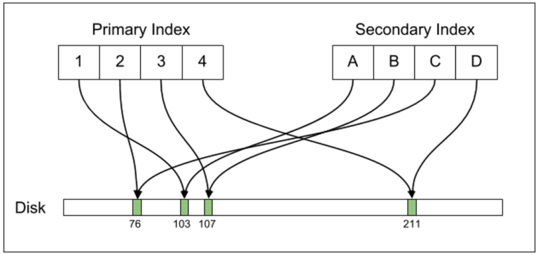
The thing to notice here is that the primary and secondary indexes each
carry record pointers to the actual records. Here's the MySQL organization
of a secondary index:
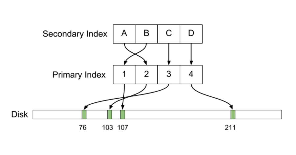
A MySQL secondary index contains pointers not to the actual records, but to
the entries in the primary index that can be used to find those records.
For read-intensive applications, the Postgres approach is faster: it
requires only one retrieval, versus two for the MySQL.
But writing and updating records complicates the picture. Suppose we update
record 103, above, so the new 103 is in a new location, perhaps to the right
of 107. For MySQL, this means we have to update the primary index, but not
the secondary index. But for Postgres, both indexes must be updated.
This phenomenon is generically known as write amplification:
one write that should be small results in multiple other writes.
(The term "write amplification" is also often used in the context of
solid-state drives; perhaps "index write amplification" would be more
specific.) It is often viewed as a consequence of having multiple indexes,
but, as we can see from the diagram, that's not exactly the case for MySQL.
Postgres has an option to reduce index write amplification known as heap-only
tuples (HOT). These work only if the update does not modify any
of the indexed attributes. For example, if there is no index on
the location field, HOT updates might work to allow regular updates of
customer locations without index manipulation. But if there is a index (eg a
GIS index), this won't work.
The simplest way to implement HOT would be by updating the tuple in
place. But this breaks multi-version concurrency control, or MVCC. We
will come to this separately, but the idea is that if transaction A updates
a tuple, then, until A completes (commits), both the original and the
A-updated tuple must remain available.
Instead, HOT must interact with the possibility of multiple tuple (record
instance) versions. Recall that Postgres keeps actual tuples in a heap
organization. An index refers to a block by its ctid pair, which points
first to the block, and then not to the record itself but to a small index
in the header of that block (the item pointer). Under HOT, this
header (or item) pointer points to the first tuple, and other tuples
representing the same record are chained together in the update chain
following the first tuple. Each separate data tuple contains indications of
which transactions are supposed to see that tuple.
In the situation of the diagrams above, what happens is that the index
points to the block header's line pointer, which in turn points to the first
tuple in the update chain. If record 103 has been updated
twice, we might have this:

The main trick to HOT is to be sure all the tuples in the chain are in the
same block. Sometimes this does fail, in which case the HOT mechanism cannot
be used for that particular update.
Eventually, unused duplicate tuples are removed via garbage collection (or vacuuming).
This itself can be a problem with very frequent updates.
HOT is applied automatically; it is not something that needs to be selected.
For more information, see www.postgresql.org/message-id/27473.1189896544@sss.pgh.pa.us.
In this blog post, rhaas.blogspot.com/2016/08/ubers-move-away-from-postgresql.html,
Postgres wizard Robert Hass acknowledges that the heap format may not always
be best:
... I believe, and have believed for a
while, that PostgreSQL also needs to be open to the idea of alternate
on-disk formats, including but not limited to index-organized formats. ...
While I'd like to hear more about Uber's experience - exactly how much
secondary index traffic did they experience and were all of those
secondary indexes truly necessary in the first place?
The bottom line here is that anyone with a million writes per second is
entitled to choose a database that is optimized for this case. Postgres is
optimized for transactions. But maybe you have a 1Mwps
load but don't need transactions. You can then choose something
else.