Comp 353/453: Database Programming, Corboy
L08, 4:15 Mondays
Week 11, Apr 8
Ch 17: basics of disks
Databases are often too big to fit everything into main memory, even today,
and disks work differently from memory, particularly when "random" access
(as opposed to linear access, below) is involved.
Disks are composed of blocks. At
the hardware level the basic unit of the sector
is typically 512 bytes, but the operating system clusters these together
into blocks of size 5K-10K. In the Elder Days applications would specify
their blocksize, but that is now very rare.
A disk looks to the OS like an array of blocks, and any block can be
accessed independently. To access a block, though, we must first move the
read head to the correct track (the
seek time) and then wait for the correct block to come
around under the head (rotational latency). Typical mean seek times are
~3-4ms (roughly proportional to how far the read head has to move, so seeks
of one track over are more like a tenth that). For rotational latency we
must wait on average one-half revolution; at 6000 rpm that is 5ms. 6000 rpm
is low nowadays, a reasonable value here is again 3-4 ms and so accessing a
random block can take 6-8ms.
Managing disk data structures is
all about arranging things so as to minimize the number of disk-block
fetches (and, to a lesser extent, minimizing the time spent on seeks). This
is a very different mind-set from managing in-memory data structures, where
all fetches are equal [ok, more-or-less equal, for those of you obsessed
with cache performance].
When processing a file linearly, a
common technique is read-ahead, or
double-buffering. As the CPU begins to process block N, the IO subsystem
requests block N+1. Hopefully, by the time the CPU finishes block N, block
N+1 will be available. Reading ahead by more than 1 block is also possible
(and in fact is common). Unix-based systems commonly begin sequential
read-ahead by several blocks as soon as a sequential pattern is observed, eg
the system reads 3-4 blocks in succession.
When handling requests from multiple processes, disks usually do not
retrieve blocks in FIFO order. Instead, typically the elevator
algorithm is used: the disk arm works from the low-numbered track
upwards; at each track, it handles all requests received by that time for
blocks on that track. When there are no requests for higher-numbered tracks,
the head moves back down.
Records can take up a variable amount space in a block; this is annoying, as
it makes finding the kth record on the block more tedious. Still, once the
block is in memory, accessing all the records is quick. It is rare for
blocks to contain more than a hundred records.
BLOBs (binary large objects) are usually not stored within records; the
records instead include a (disk) pointer to the BLOB.
File organizations
The simplest file is the heap file,
in which records are stored in order of addition. Insertion is efficient;
search takes linear time. Deletion is also slow, so that sometimes we just
mark space for deletion.
Another format is to keep the records ordered (sorted) by some field, the ordering field. This is not necessarily
a key; for example, we could keep file Employee ordered by Dno. If the
ordering field is a key, we call it the ordering
key. Ordered access is now fast, and search takes log(N) time
(where N is the length of the file in
blocks and we are counting only block accesses). Note that the
actual algorithm for binary search is slightly different from the classic
array version: if we have blocks lo
and hi, and know that the desired
value X must, if present, lie between these two blocks, then we retrieve the
block approximately in between, mid.
We then check to see one of these cases:
- X < key of first record
on block mid
- X > key of last record on
block mid
- X is between the keys, inclusive, and so either the record is on
block mid or is not found
Note also that the order relation used to order the file need not actually
have any meaning terms of the application! For example, logically it makes
no sense to ask whose SSN is smaller. However, storing an employee file
ordered by SSN makes lookups by SSN much faster.
See Fig 17.7
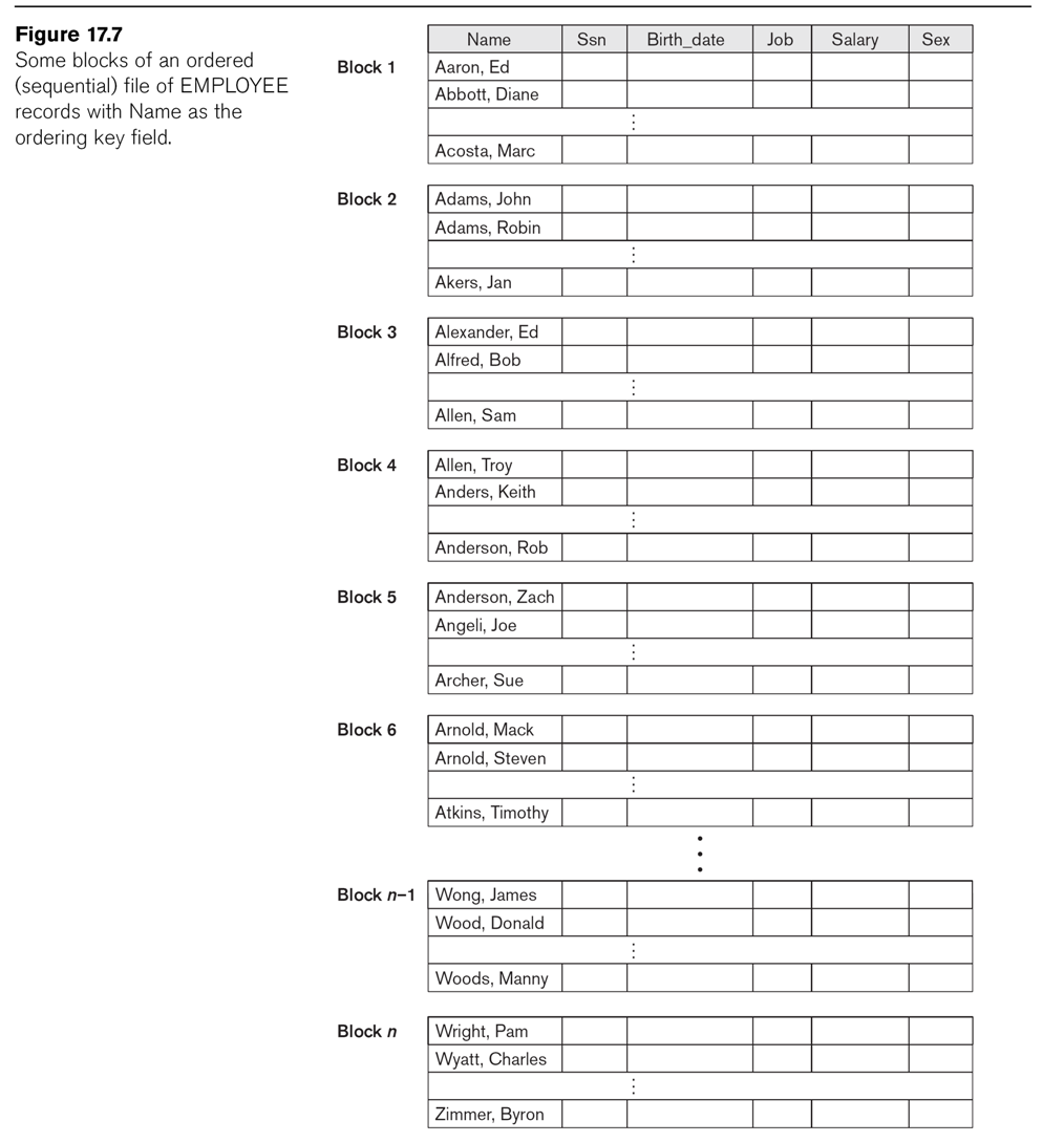
Insertion and deletion are expensive. We can improve insertion by keeping
some unused space at the end of each block for new records (or the
moved-back other records of the block). We can improve deletion by leaving
space at the end (or, sometimes, right in the middle).
Another approach is to maintain a transaction
file: a sequential file consisting of all additions and deletions.
Periodically we update the master file with all the transactions, in one
pass.
Hashing
Review of internal
(main-memory-based) hashing. We have a hash function h that applies to the
key values, h = hash(key).
- bucket hashing: the hash table component hashtable[h] contains a
pointer to a linked list of records for which hash(key) = h.
- chain hashing: if object Z hashes to value h, we try to put Z at
hashtable[h]. If that's full, we try hashtable[h+1], etc.
For disk files, we typically use full blocks as buckets. However, these will
often be larger than needed. As a result, it pays to consider hash functions
that do not generate too many different values; a common approach is to
consider hash(key) mod N, for a smallish N (sometimes though not universally
a prime number).
Given a record, we will compute h = hash(key). We also provide a
single-block map ⟨hash,block⟩ of hash values to block addresses (in effect
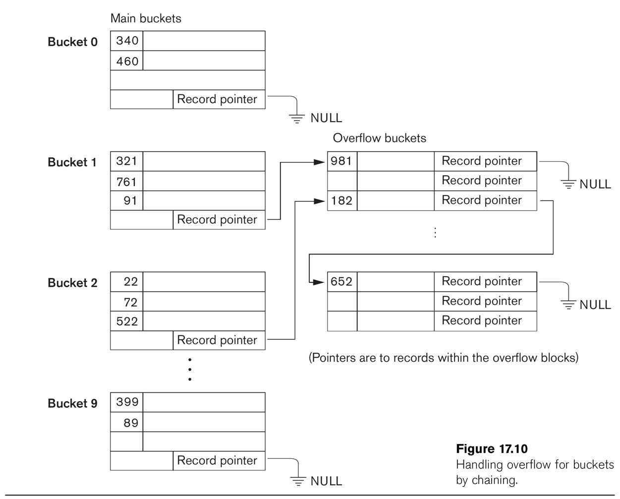
corresponding to hashtable[]). Fig 17.9 shows the basic strategy. More
detail on the buckets is provided in Fig 17.10, which also shows some
overflow buckets; in this diagram, the hash function returns the last digit
of the key-field value (eg hash(127) = 7). Note that Bucket 1 and Bucket 2 share an overflow bucket; we also can
(and do) manipulate the ⟨hash,block⟩ structure so that two buckets share a
block (by entering ⟨hash1,block1⟩ and ⟨hash2,block2⟩ where block1 = block2).
When a single bucket approaches two blocks, it can be given its own overflow
block.
When more than one bucket shares an overflow bucket, it is likely we will
keep some expansion space between the two sets of records.
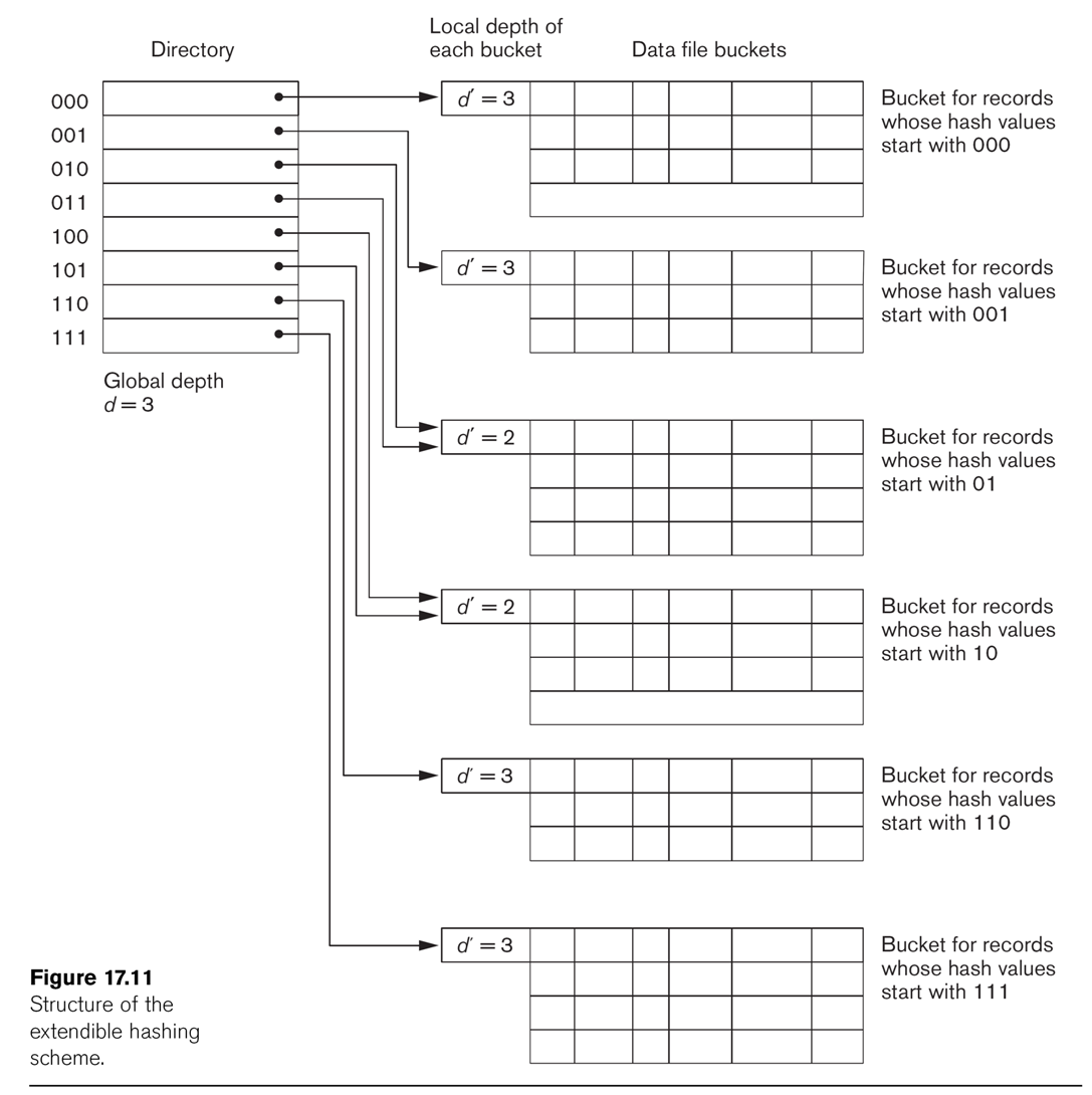
Extendible Hashing
This technique manages buckets more efficiently. We hash on the first d bits of the hash values; d is called
the global depth. We keep a
directory of all 2d possible values for these d bits, each with a
pointer to a bucket block. Sometimes, two neighboring buckets are consolidated
in the directory; for example, if d=3, hash prefix values 010 and 011 might
point to the same block. That block thus has a reduced local
depth of 2.
As we fill blocks, we need to create new ones. If a block with a reduced
local depth overflows, we split it into two blocks with a greater depth
(still ≤ d). If a block with local depth d overflows, we need to make some
global changes: we increment d by 1, double the directory size, and double
up all existing blocks except for the one causing the overflow.
For this to work well, it is helpful to have a hash function that
is as "pseudorandom" as possible, so for any prefix-length d the 2d
buckets are all roughly the same size. (The size inequality can be pretty
rough; even with perfect randomness the bucket sizes will be distributed
according to the Poisson distribution).
See Fig 17.11.
Extendible hashing grew out of dynamic
hashing, in which we keep a tree structure of hashcode bits,
stopping when we have few enough values that they will all fit into one
block.
Ch 18: indexing
It is common for databases to provide indexes
for files. An index can be on either a key field or a non-key field; in the
latter case it is called a clustering
index. The index can either be on a field by which the file is
sorted or not. An index can have an entry for every
record, in which case it is called dense;
if not, it is called sparse. An
index on a nonkey field is always considered sparse, since if every record
had a unique value for the field then it would in fact be a key after all.
A file can have multiple indexes, but the file itself can be structured only
for one index. We'll start with that case. The simplest file structuring for
the purpose of indexing is simply to keep the file sorted on the attribute
being indexed; this allows binary search. For a while, we will also keep
restrict attention to single-level indexes.
Primary Index
A primary index is an index on the
primary key of a sorted file (note
that an index on the primary key, if the file is not maintained as sorted on
that primary key, is thus not a
"primary index"!). The index consists of an ordered list of pairs ⟨k,p⟩,
where k is the first key value to appear in the block pointed to by p (this
first record of each block is sometimes called the anchor
record). To find a value k in the file, we find consecutive ⟨k1,p⟩
and ⟨k2,p+1⟩ where k1≤k<k2; in that case, the record with key k must be
on block p. This is an example of a sparse
index. A primary index is usually much smaller than the file
itself. See Fig 18.1.
Example 1 on EN6 p 635: 30,000 records, 10 per block, for 3000 blocks.
Direct binary search takes 12 block accesses. The index entries are 9+6
bytes long, so 1024/15 = 68 fit per 1024-byte block. The index has 3000/68 =
45 blocks; binary search requires 6 block accesses, plus one more for the
actual data block itself.
Clustering index
We can also imagine the file is ordered on a nonkey field (think
Employee.dno). In this case we create a clustering
index. The index structure is the same as before, except now the
block pointer points to the first block that contains any records with that
value; see Fig 18.2. Clustering indexes
are of necessity sparse. However, it is not necessary to include in the
index every value of the attribute; we only need to include in the index the
attribute values that appear first in each block. But there's a tradeoff; if
we skip some index values then we likely will want an index entry for every
block; for a non-key index this may mean many more entries than an index
entry for every distinct value. In Fig 18.2, we have an entry for
every distinct value; we could remove the entries for Dept_number=2 and
Dept_number=4.
Another approach to clustering indexes may be seen in Fig
18.3, in which blocks do not contain records with different cluster
values. Note that this is again a method of organizing the file
for the purpose of the index.
Ordering a file by a nonkey field may sound unlikely. However, it may be
quite useful in cases where the file has a multi-attribute key. For example,
we might keep the works_on file ordered by essn; the essn alone is not a
key. This would allow easy lookup of any employee's projects. We might in
fact keep the file ordered lexicographically by the full key, ⟨essn,pno⟩, in
which case the file would be automatically ordered by essn alone,
and we could create a clustering index on essn alone. Yet another example of
a plausible clustering index is the invoice_item file we considered
previously. The key is ⟨invoice_num, partnum⟩. Keeping the file ordered
first by invoice_num and second by partnum would allow a clustering index on
invoice_num alone, which is likely to be something we frequently need to do.
(This example is in some sense the same as the works_on example.)
Secondary Indexes
Now suppose we want to create an index for Employee by (fname, lname),
assumed for the moment to be a secondary key.
The record file itself is ordered by SSN. An index on a secondary
key will necessarily be dense, as the file won't be ordered by the
secondary key; we cannot use block anchors. A common arrangement is simply
to have the index list ⟨key,block⟩ pairs for every key value appearing; if
there are N records in the file then there will be N in the index and the
only savings is that the index records are smaller. See Fig
18.4. If B is the number of blocks in the original file, and BI is the
number of blocks in the index, then BI ≤B, but not by much, and log(BI) ≃
log(B), the search time. But note that unindexed search is linear
now, because the file is not ordered on the secondary key.
Example 2, EN6, p 640: 30,000 records, 10 per block. Without an index,
searching takes 3,000/2 = 1500 blocks on average. Blocks in the index hold
68 records, as before, so the index needs 30,000/68 = 442 blocks; log2(442)
≃ 9.
Secondary indexes can also be created on nonkey
fields. We can create dense indexes as above, but now with multiple entries
for the indexed attribute, one for each record (Option 1 in EN6 p 640). A
second approach (option 2 in EN6 p 640) is to have the index consist of a
single entry for each value of the indexed attribute, followed by a list
of record pointers. The third option, perhaps the most common, is for each
index entry to point to blocks of
record pointers, as in Fig 18.5.