Comp 353/453: Database Programming, Corboy
L08, 4:15 Mondays
Week 5, Feb 18
Read in Elmasri & Navathe (EN)
- Chapter 4: Basic SQL
- Chapter 5: More-complex SQL (section 5.1 especially)
GROUP BY and HAVING
Recall Query 25 from last week: for each project, give the project number,
the project name, and the number of employees who worked on it. Our solution
was the following:
select p.pnumber, p.pname, count(*) as
employees
from PROJECT p, WORKS_ON w
where p.pnumber = w.pno
group by p.pnumber, p.pname
In this query, we listed the project number, project name and employee count
for each project. Suppose we want (Query 26)
this information for each project with
more than two employees. We introduce the having
clause, which works like the where
clause but is used to select entire groups.
select p.pnumber, p.pname,
count(*)
from PROJECT p, WORKS_ON w
where p.pnumber = w.pno
group by p.pnumber, p.pname
having count(*) > 2;
Note that we first apply the where
clause to build the "ungrouped" table, and then apply the group
by clause to divide the rows into groups, and finally restrict the
output to only certain groups by using the having
clause. Any aggregation functions in the having clause
work just as they would in the select clause: they
represent aggregation over the individual groups. In the case above,
count(*) represents the count of each group.
Here's another example (query 27):
for each project, retrieve the project number & name, and the number of
dept-5 employees who work on it. E&N's solution is here:
select p.pnumber, p.pname,
count(*)
-- WRONG
from PROJECT p, WORKS_ON w, EMPLOYEE e
where p.pnumber = w.pno and w.essn = e.ssn and e.dno = 5
group by p.pnumber, p.pname;
This is actually wrong, if you interpret it as wanting all
projects even if there are zero
dept-5 employees at work on them. With the default data, project 30
(Newbenefits) is in this category. The problem is similar to that solved by
outer joins: if there are no dept-5 employees on the project, then no join
row is created at all.
Problem: GROUP BY will never include
empty groups. If you want to include groups with count(*) =
0, use an inner query
This is an important point. Let's leave out the count(*) and the group
by (and add an order by p.pnumber);
the result of the query is:
+---------+-----------------+
| pnumber | pname           |
+---------+-----------------+
|       1 | ProductX        |
|       1 | ProductX        |
|       2 | ProductY        |
|       2 | ProductY        |
|       2 | ProductY        |
|       3 | ProductZ        |
|       3 | ProductZ        |
|      10 | Computerization |
|      20 | Reorganization  |
+---------+-----------------+
Doing the grouping manually, we see that we have groups of sizes 2
(pnumber=1), 3 (pnumber=2), 2, 1 and 1, as expected. But
there are no groups of size zero shown!
Here is a working version:
select p.pnumber, p.pname,
(select count(*) from WORKS_ON w, EMPLOYEE
e
where p.pnumber = w.pno and w.essn = e.ssn and e.dno = 5) as dept5_count
from PROJECT p
;
This technique can often be used to write a query involving group
by as one without.
(Why did I introduce the column name dept5_count here?)
Another group-by/having issue is
illustrated in Query 28: give the
number of employees in each department whose salaries exceed $40,000, but
only for departments with more than five employees. In order to get a
nonempty result, let's change this to $29999 and >2 employees. The book
gives the following wrong version
first (correctly identifying it as wrong!):
select d.dname, count(*) as
highpaid
-- WRONG
from department d, employee e
where d.dnumber = e.dno and e.salary > 29999
group by d.dname
having count(*) > 2;
Note that the Administration department has three employees, with the
following salaries; the department has >2 employees and there is one with
a salary > 29999:
+----------+---------+----------+
| Alicia   | Zelaya  | 25000.00 |
| Jennifer | Wallace | 43000.00 |
| Ahmad    | Jabbar  | 25000.00 |
+----------+---------+----------+
What shows up in the output of the query above? Recall that the where
clause is evaluated at the beginning; if we put the salary constraint there,
then we ignore employees making less than that, and thus potentially
undercount some departments.
Problem: count(*) always counts the
same thing, in a query, whether it is in the select clause or the having
clause. If, as here, you want count(*) to mean one thing in one place
(count of dept employees with high salary) and
another thing in another place (count of all
dept employees), you need an inner query.
Here is a working version (actually, the book's version of this is
syntactically broken, as they left out the "e.dno in"; I think this is a
typo rather than a design error).
select d.dnumber, d.dname,
count(*) as highpaid
from department d, employee e
where d.dnumber = e.dno and e.salary > 29999 and
e.dno in
(select e.dno from employee e group
by e.dno having count(*)
> 2)
group by d.dnumber, d.dname;
Another ALL example
List departments that
are at all locations
This doesn't mean every location in the world; it means all the locations in
the list
select distinct dlocation from dept_locations;
First of all, if we try
select distinct dlocation from dept_locations;
we get the list Houston, Stafford, Bellaire, Sugarland. But if we query
select * from dept_locations
we get
+---------+-----------+
|       1 | Houston   |
|       4 | Stafford  |
|       5 | Bellaire  |
|       5 | Houston   |
|       5 | Sugarland |
+---------+-----------+
No department is at every location (dept 5 is not at Stafford). So to have a
nonempty result, we have to insert a record:
insert into dept_locations values(5, 'Stafford');
delete from dept_locations where dnumber = 5 and
dlocation = 'Stafford';
If we want two entries, we can
insert into dept_locations values (1, 'Stafford'), (1,
'Bellaire'), (1, 'Sugarland');
delete from dept_locations where dnumber = 1 and
dlocation in ('Stafford',
'Bellaire', 'Sugarland');
As we did last week, we will approach "departments d at all locations" by
first changing to the equivalent "departments d for which there does not
exist a location that d is not located at", or "departments d for which
there does not exist a location L such that d is not located at L".
The next step is to transform "d is located at L" to SQL:
exists (select * from dept_locations loc2 where
loc2.dnumber = d.dnumber and loc2.dlocation = L)
(locations L are simple strings, not some larger record as department
d was). To change this to "d is not
located at L", we just change exists
to not exists. I used the name
"loc2" because the outer query will use name loc1.
We now say "there does not exist a location L such that d is not located at
L" as
not exists (select * from dept_locations
loc1 where not exists
(select * from dept_locations loc2 where
loc2.dnumber = d.dnumber and loc2.dlocation =
loc1.dlocation))
The italicized part is the parenthesized part of the previous query, still
with d a free variable but with L replaced by loc1.dlocation.
To finish it off, we put "select d.dno from department d where" in front of
it:
select d.dnumber from department d where not
exists (select * from dept_locations loc1 where not exists
(select * from dept_locations loc2 where
loc2.dnumber = d.dnumber and loc2.dlocation = loc1.dlocation))
The italicized part here is the entire previous query, with d no longer free
(why?)
This looks circular, or like the loc2 name is redundant, but it's not: the
loc2 record refers to a possible location of department d; loc1 refers to
any other location.
- "There is no location loc1 for which there is no location loc2 of d
that is equal to loc1", or
- "There is no location loc1 which is not a location of d".
Another way to look at this is that for every loc1 (every possible location)
there is a loc2 at the same
location that matches d.
Triggers
Chapter 4 had two uses of the CHECK statement (neither of which we did at
the time): attribute checks and record checks.
Two further checks are assertions
and triggers. These sometimes have
efficiency consequences, however.
1. Attribute checks
example: for the department table,
dnumber INT not null check
(dnumber >0 and dnumber < 100)
These are applied whenever an individual attribute is set.
Here's another important attribute check (MySQL syntax)
create table employee2 (
name varchar(50) not null,
ssn char(9) primary key not null,
dno INT not null check (dno > 0 and dno
< 100),
check (ssn RLIKE
'[0-9][0-9][0-9][0-9][0-9][0-9][0-9][0-9][0-9]')
) engine innodb;
We can populate this from table employee:
insert into employee2
select e.lname, e.ssn, e.dno from employee e;
Some additional insertions that should fail:
insert into employee2 values ('anonymous',
'anonymous', 37);
insert into employee2 values ('joe hacker', '12345678O',
37); // that is the letter 'O'
insert into employee2 values ('jack hack', '12345689',
25); // not enough
digits
They do not fail! MySQL ignores checks (even on dno). Actually, MySQL does
not even check that there are parentheses around the body of the check
condition.
How about postgres?
create table employee2 (
name varchar(50) not null,
ssn char(9) primary key not null,
dno INT not null check (dno > 0 and dno
< 100),
check (ssn SIMILAR TO
'[0-9][0-9][0-9][0-9][0-9][0-9][0-9][0-9][0-9]')
);
This should work.
You can also do this in postgres:
create table employee3 (
name varchar(50) not null,
ssn char(9) primary key not null,
dno INT not null check (dno > 0 and dno
< 100),
check (char_length(ssn)
= 9)
);
2. Record (tuple) checks
create table DEPARTMENT (
dname ....
dnumber ...
mgr_ssn ...
mgr_start
DATE not null,
dept_creation
DATE not null,
check
(dept_creation <= mgr_start)
);
These are applied whenever a particular row is updated or added to that
table.
3. Assertions
Assertions are general requirements on the entire
database, to be maintained at all times.
create assertion salary_constraint
check ( not exists
(select * from employee e, employee s,
department d
where e.salary > s.salary and e.dno = d.dnumber and d.mgr_ssn =
s.ssn)
);
The problem with this (aside from the fact that this is not
always a good business idea) is when and where it is applied. After every
database update? But only some updates even potentially result in
violations: changes to employee salaries, and changes of manager.
From the manual:
PostgreSQL does not
implement assertions at present.
4. Triggers
Due to the "expense" of assertions, some databases (eg Oracle) support triggers: assertions that are only
checked at user-specified times (eg update or insert into a particular
table).
create trigger salary_violation
before insert or update of
salary, super_ssn on employee
for each row when (new.salary >
(select salary from employee e
where e.ssn = new.super_ssn))
inform_supervisor
(New.supervisor_ssn, new.ssn) --
some prepared external procedure
);
In postgres, we'd finish off with
for each row execute
procedure inform_supervisor);
That is, we can't have the when
clause.
Writing the external procedures is beyond the scope of SQL.
VIEWS
Here's a simple view, that is, a
sort of "virtual table". The view is determined by the select
statement within. The point, though, is not
that we set works_on1 here to be
the output of the select, but that
as future changes are made to the underlying tables, the view is
automatically updated.
create view works_on1 AS
select e.fname, e.lname, p.pname, w.hours
from employee e, project p, works_on w
where e.ssn = w.essn and w.pno= p.pnumber;
We can now do:
select * from works_on1;
select w.lname, sum(w.hours)
from works_on1 w
group by w.lname;
Now let's add an employee:
insert into employee values ('Ralph', null, 'Wiggums', '000000001',
'1967-03-15', null, 'M', 22000, '333445555', 5);
insert into works_on values ('000000001', 1, 9.8);
Ralph is there (working on 'ProductX'). To delete:
delete from works_on where essn='000000001';
delete from employee where ssn='000000001';
Here's a typical use of views for a single
table: hiding some columns (I've hidden salary
for privacy reasons, and address
for space):
create view employee1 AS
select fname, minit, lname, ssn, bdate, sex, super_ssn, dno from employee;
Finally, here's another example from the book, demonstrating column renaming
and use of aggregation columns:
create view deptinfo (dept_name,
employee_count, total_salary) AS
select d.dname, count(*), sum(e.salary)
from department d, EMPLOYEE e
where d.dnumber = e.dno
group by dname;
There are two primary implementation strategies for views:
- query rewriting
- materialization
It is typically a problem to update views, though we can do this for the
employee1 view so long as the missing fields do not have not
null constraints (and also that we include the underlying employee
table's primary key in the view).
In creating mailing lists for Microsoft Access, a given list is based not on
a query (which would make the most
sense), but on a named view.
Schema change
We've already seen ALTER TABLE in use: we used it to add foreign key
constraints after some initial values were entered:
alter table employee add foreign key (dno)
references department(dnumber);
Another application is for schema changes as the database needs evolve.
Oracle ROWNUM
Oracle allows the use of the "virtual" column rownum
when working with sorted tables. This way one can print the third-highest
value, for example (where rownum = 3),
or the top 10 values (where rownum <=10).
Relational Algebra
We'll only do a quick look at this. The point is that SQL has a precise
mathematical foundation; this allows the query
optimizer to rewrite queries (ie to prove that
alternative forms of some queries are equivalent).
First some set-theoretic notations:
Union: R1 ∪ R2, where R1, R2 are subsets of same cross product (that
is, they are sets of tuples of the same type). This is logically like OR
Intersection: Logically like AND
Difference: Logical "R1 but NOT R2"
R1 − R2
The basic relational operations are:
PROJECTION: selecting some designated columns, ie taking some vertical
slices from a relation. Projection corresponds to the select
col1, col2, etc part of the query. It is denoted with π, subscripted with
column names: πlname,salary(R).
SELECTION: Here we specify a Boolean condition that selects only some rows
of a relation; this corresponds to the where
part of a SQL query
- choosing subset of entries
- corresponds to logical operations defining the subset
- Sel(Parts:cost >10.0)
This is denoted by σ, subscripted with the condition: σdno=5 AND
salary>=30000(R)
More examples can be found on pp 147-149 of E&N.
PRODUCT: The product R×S is the set of ordered pairs {⟨r,s⟩ | r∈R and s∈S}.
The product can be of two tables (relations) as well as of two
domains; in this case, if r=⟨r1,r2,...,rn⟩
and s=⟨s1,s2,...,sk⟩, then we likely
identify the pair ⟨r,s⟩ with the n+k-tuple ⟨r1,r2,...,rn,s1,s2,...,sk⟩.
JOIN
The join represents all records from table R and table S where R.colN =
S.colM
The traditional notation for this is R⋈S, or, when we wish to make the join
condition explicit, R⋈colN=colMS. If the join column has the same
name in both R and S, we may just subscript with that column name: R⋈ssnS.
The join can be expressed as Product,Selection,Projection as follows:
πwhatever cols we need to keep (σcolN=colM(R×S))
In other words, the join is not a "fundamental" operation; contrast this
with the "outer join" below. As a suggestion for implementation,
the above is not very efficient: we never want to form the entire product
R×S. But this notation lets us restructure the query for later optimization.
The equijoin
is a join where the join condition involves the equality operation; this is
the most common.
The natural join is a join where we
delete one of the two identical columns of an equijoin. That is, if R is
⟨ssn,lname⟩ and S is ⟨ssn, proj⟩, then the equijoin is really
⟨ssn,lname,ssn,proj⟩, where the two ssns are equal, and the natural join is
⟨ssn,lname,proj⟩.
Note that the outer join can not be expressed this way; the outer
join of two relations R and S is not necessarily a subset of R×S (though it
may be subset of R×(S ∪ {NULL}). The outer join is fundamentally about
allowing NULL values. If foo is the
name of the join column in R, the outer join is of the form
R⋈S ∪ (σfoo∉π_foo(S)
(R) × {NULL})
(Explain)
Note the condition here is strictly speaking outside the scope of the
Boolean expressions at the bottom of page 147 of E&N.
Division: R ÷ S: As above, we
identify R with a relation T×S; R÷S is then {t∈T| ∀s∈S ⟨t,s⟩∈R} ("∀s∈S"
means "for all s in S"). In English, which records in T appear combined with
EVERY row of S.
As an example, let E be the employees table, and P be the projects, and W be
the Works_on table, a subset of E×P. Then W ÷ P is the set of employees who
have worked on every project; W ÷ E is the set of projects worked on by
every employee. Note the implicit "closed world" hypothesis: we're only
considering project numbers (or employee numbers) that actually appear in P
and E.
Note the prerequisite that R is a table "extending" that of S: R has all the
columns that S has, and more. The underlying set of columns of R ÷ S is the
set (columns of R) − (columns of S). It is usually easier to think of
division as being of the form T×S ÷ S.
Asking which students got only A's is not
quite an example of this (why?)
The book also defines a rename
operation; for certain purposes this is important but I classify it as
"syntactic sugar".
The book also uses an assignment operator (TEMP ← σcolN=colM(R×S)).
However, we can always substitute the original expression in for the TEMP
variable.
Query trees
Here is figure 6.9 from EN6 page 165. The question is for
every
project located in Stafford, list the project number, the controlling
deparment number, and the department manager's last name, address and
birth date. In SQL this is.
select p.pnumber, p.dnum,
e.lname, e.address, e.bdate
from project p, department d, employee e
where p.dnum = d.dnumber and d.mgr_ssn = e.ssn and p.plocation =
'Stafford'
Here is this query in a query-tree representation:
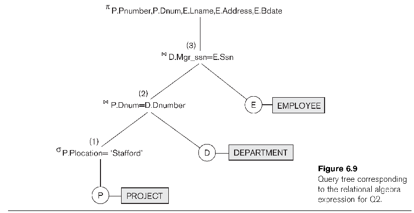
Note that the tree allows us to express the solution as a SEQUENCE of steps.
Another double-join example, listing employees and the projects they worked
on.
Select e.lname, p.pname from employee e,
works_on w, project p
where e.ssn = w.essn and w.pno = p.pnumber;
Entity-Relationship modeling
This is a variant (actually a predecessor) of object modeling (eg UML or CRC
cards or Booch diagrams). In the latter, everything is an object. In ER
modeling, we will make a distinction between entities
(things) and relationships. As a
simple example, students and courses are entities; but the enrolled_in
table is a relationship. Sections most likely would be modeled as entities
too, though there is a relationship to COURSE.
The ER process starts, like most software-engineering projects, with
obtaining requirements from users. What data needs to be kept, what queries
need to be asked, and what business rules do we build in? (For example, if
the DEPARTMENT table has a single column for manager, then we have just
committed to having a single manager for each department.)
The goal of the E-R modeling process is to create an E-R
diagram, which we can then more-or-less mechanically convert to a
set of tables. Both entities and relationships will correspond to tables;
entity tables will often have a single-attribute primary key while the key
for relationship tables will almost always involve multiple attributes.
Here is an E-R diagram for the OFFICE database. (The figure below was
Fig 3.2 in an earlier edition of E&N; it is Fig 7.2 in the 6th edition.)
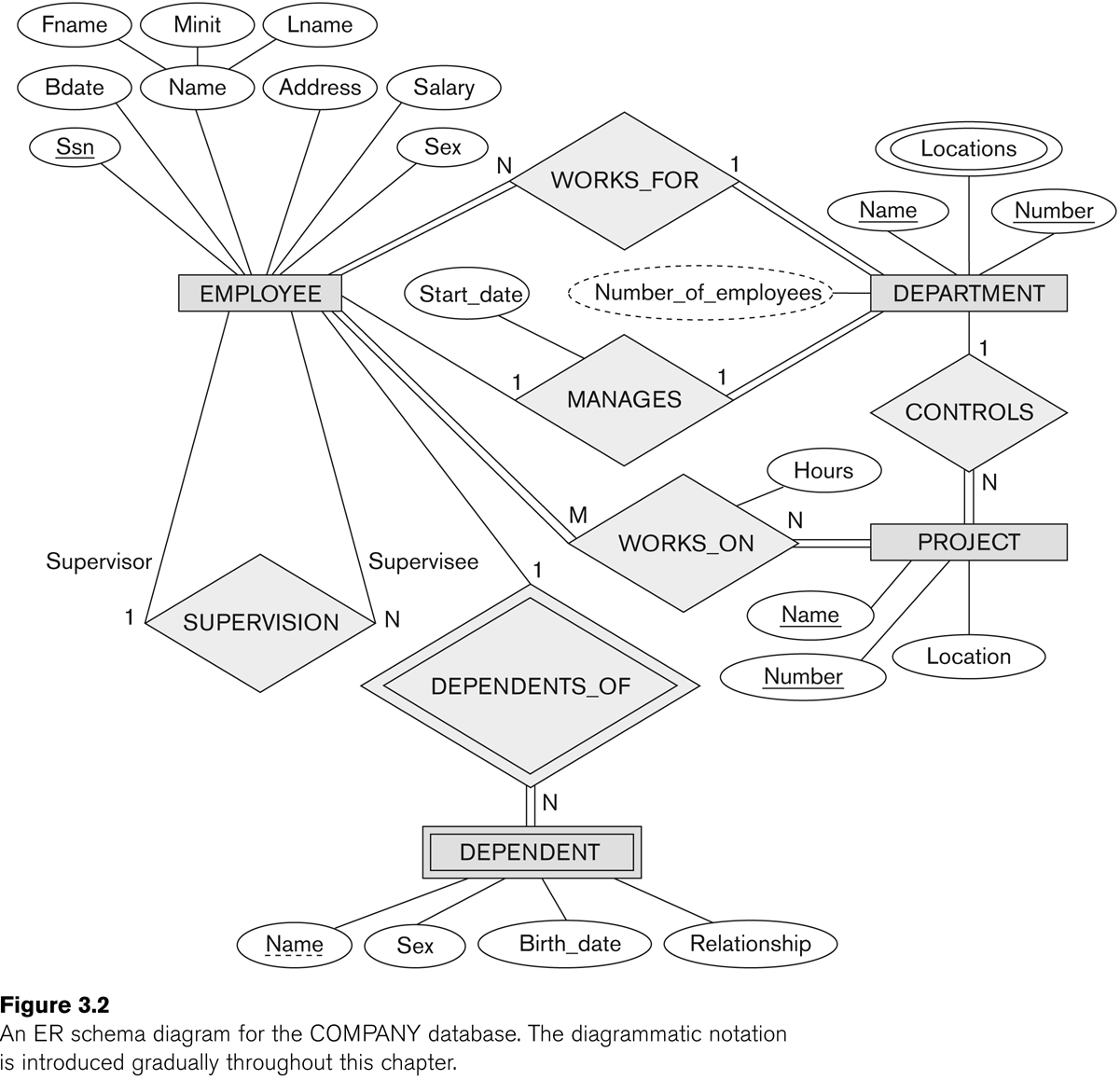
Entities
After the above beginnings, we identify the entities.
These should represent physical things, such as employees or parts or (more
abstractly) departments. Note that customer_orders might be modeled as an
entity, but might also be modeled as a relationship.
Entities have attributes, which
will later more or less become the fields. For each attribute we have the
following aspects:
- composite v single: a social-security number is a single attribute; an
address (consisting of street, apt, city, state, zip) would be
composite. So would a name.
- single-valued v multi-valued: E&N's examples here are
college_degrees and vehicle_color.
- stored v derived: the classic derived attribute is age, derived from
birthdate.
We also must decide which attributes can be NULL.
Attributes at this point should not be references to other tables; instead,
we will create those references when we create relationships.
The book uses () to represent sub-attributes of composite attributes, and {}
to surround multi-valued attributes.
Traditionally we represent the entity with a rectangular box, and the
attributes are little oval tags.
An entity type is our resulting
schema for the entity; the entity set
is the actual set of entities.
In the diagram, we will underline
the key attributes. If a key is composite, say (state,regnum), then we make
a composite attribute out of those pieces.
This is a slight problem if the key can be either (state,regnum) or
(state,license_plate); how could we best address this?
Note that key attributes really represent constraints.
In the early stages, we allowed entity attributes to be composite or
computed or multi-valued; all of these will eventually be handled in
specific ways as we translate into SQL.
Often there is more than one way to do things. In the COMPANY example, we
might list dept as an attribute of
EMPLOYEE, and eventually conclude that because dept
represented an instance of another entity (DEPARTMENT), we would have a
foreign-key constraint on EMPLOYEE.dept, referring to DEPARTMENT.dnumber.
Note, however, that we could
instead list employees as a
multi-valued attribute of DEPARTMENT. One reason for not doing this is that
we do want to minimize the use of multi-valued attributes, but this
arrangement would have been a possible option. Later, we even could implement
this second approach by adding an attribute dept
to the EMPLOYEE table (the table, not entity).
We actually could have both forms,
but we would need to understand the constraint that if employee e is in the
employees multi-valued attribute for
DEPARTMENT d, then department d must be be the value of the EMPLOYEE e's dept attribute. That is, the dual
attributes would have to be inverses.
As for naming entities, a common practice (used by E&N) is to name them
with singular nouns. Nouns because they should represent things; singular
for the individual objects. Eventually we will have a table of employees, plural, but we call it EMPLOYEE to
represent what entities it contains.
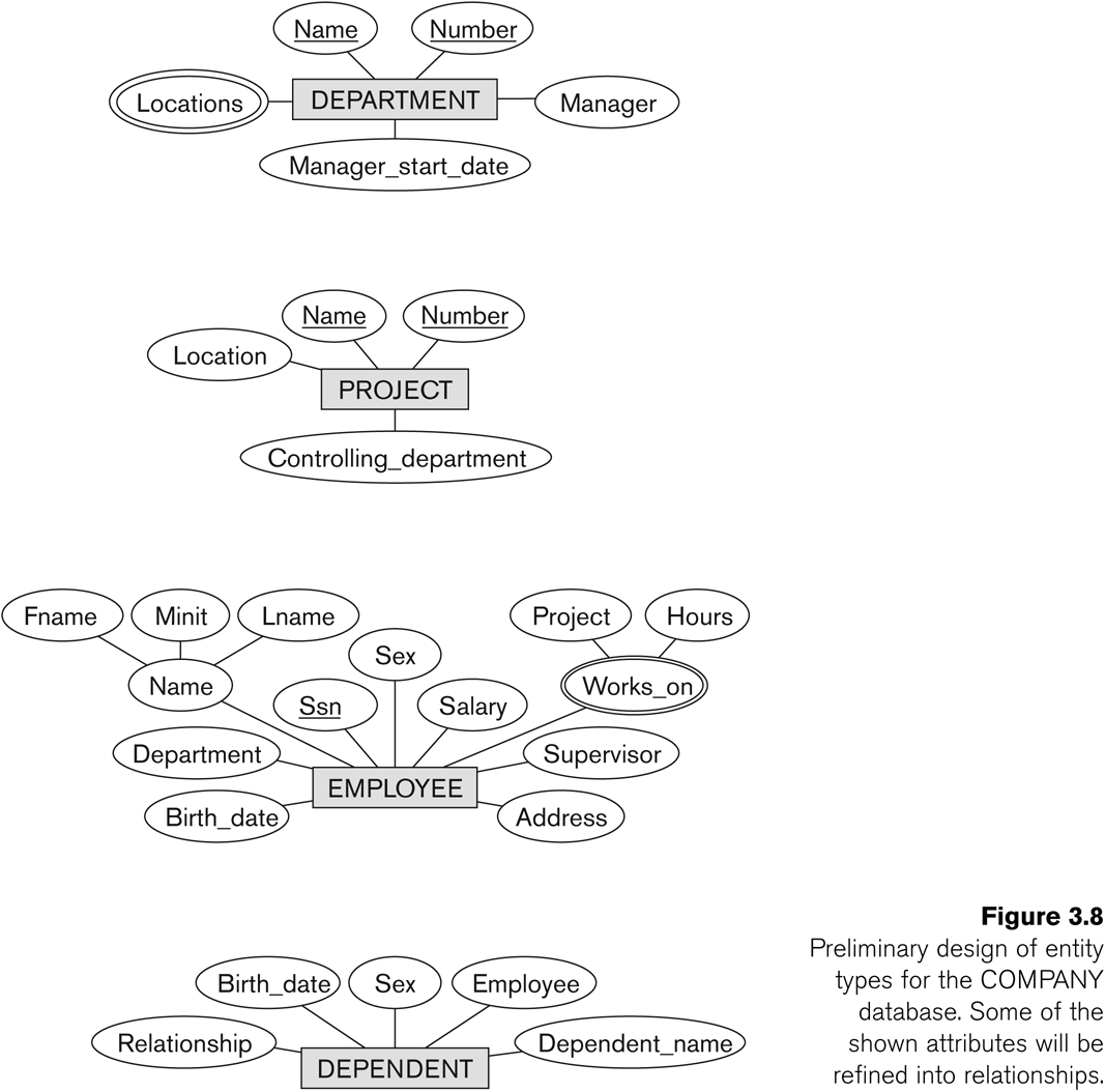
Weak entities
The usual definition of a weak entity is that it is an entity that does not
have key attributes of its own. The classic example is the DEPENDENT entity,
with attributes name, birth_date,
sex and relationship;
a dependent is uniquely determined by the name
and the employee to whom the dependent is associated. You might wonder why
we don't add an attribute employee
at the beginning, and have ⟨name, employee⟩ be the key. One problem with
that approach is that employee is a
reference to a different entity; such references should really be described
as relationships. After all, the EMPLOYEE is really someone else, not an
attribute of the DEPENDENT person itself (at least not in the same sense as
bdate, age, etc). We will say, instead, that there is a relationship
between the DEPENDENT entity and EMPLOYEE; this relationship is the identifying
relationship for DEPENDENT.
In general, during the design process, the statement that "dependents do not
have a key" is subject to interpretation; we can
always declare that the associated employee's SSN is part of the key.
However, the point is that dependents do not have a "natural" key that is an
attribute of the dependent itself. Also, using the "employee_ssn" as an
attribute is suspect because it realistically is an attempt to refer to
another table.
There is a total participation constraint
between DEPENDENT and EMPLOYEE; every DEPENDENT must be connected to some
EMPLOYEE. As the book points out, however, every DRIVERS_LICENSE is
associated with some PERSON, but the DRIVERS_LICENSE entity does in fact
have its own key: the drivers_license_number.
The way that DEPENDENT could become a strong entity is if we added its own key: dependent_ssn. But typically
the SSNs of dependents are not known (minor dependents may not even have
SSNs), so we choose not to implement the database this way.
The DEPENDENT entity does have a partial
key: the attribute name,
which, together with the associated EMPLOYEE object, does define a key.
We could also represent dependents
as a multi-valued, composite attribute of EMPLOYEE.
Fig 7.8 (6th-edition numbering) lists all the entities: