Comp 353/453: Database Programming, Corboy
523, 7:00 Thursdays
Week 11, Apr 13
Read in Elmasri & Navathe (EN)
- Chapter 15, Normalization
- PHP and debugging
- lamp.cslabs.luc.edu
A superkey (or key superset) of a relation schema
is a set of attributes S so that no two tuples of the relationship can
have the same values on S. A key
is thus a minimal superkey:
it is a superkey with no extraneous attributes that can be removed. For
example, {Ssn, Dno} is a superkey for EMPLOYEE, but Dno doesn't matter
(and in fact contains little information); the key is {Ssn}.
Note that, as with FDs, superkeys are related to the sematics of the
relationships, not to particular data in the tables.
Relations can have multiple keys, in which case each is called a candidate key.
For example, in table DEPARTMENT, both {dnumber} and {dname} are
candidate keys. For arbitrary performance-related reasons we designated
one of these the primary key;
other candidate keys are known as secondary
keys.
A prime attribute is an
attribute (ie column name) that belongs to some candidate key. A nonprime
attribute is not part of any key.
A dependency X⟶A is full if
the dependency fails for every proper subset X' of X; the dependency is
partial if not, ie if there is a proper subset X' of X such
that X'⟶A.
2NF: If K represents the set of
attributes making up the primary key, every nonprime
attribute A (that is an attribute not a member of any key) is
functionally
dependent on K (ie K⟶A), but that this fails for any proper subset of K
(no proper subset of K functionally determines A).
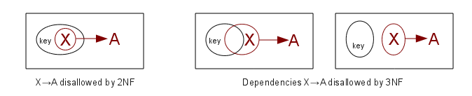
3NF: 2NF + there is no dependency X⟶A for nonprime attribute A and for an attribute
set X that does not contain
a key (ie X is not a superkey).
Consider the LOTS example of Fig 15.12.
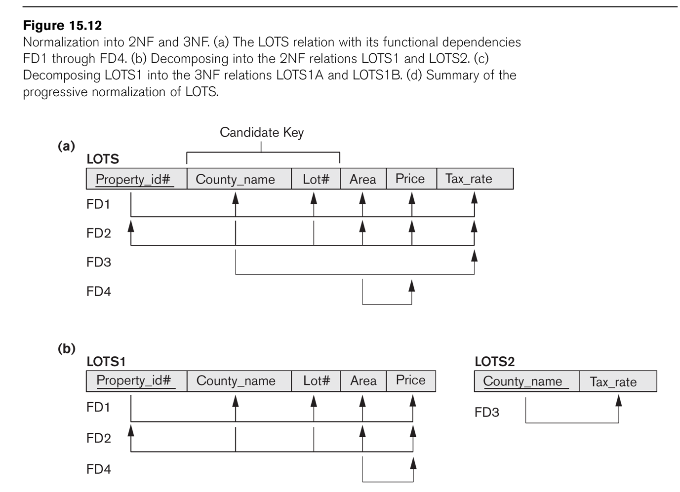
Attributes are
- property_ID
- county
- lot_num
- area
- price
- tax_rate
Third Normal Form
Third Normal Form (3NF) means that the relation is in 2NF and also
there is no dependency X⟶A for nonprime attribute A and for attribute
set X that does not contain
a candidate key (ie X is not a superkey). In other words, if X⟶A holds
for some nonprime A, then X must be a superkey. (For comparison, 2NF
says that if X⟶A for nonprime A, then X cannot be a proper subset of
any key, but X can still overlap with a key or be disjoint from a key.)
If X is a proper subset of a key, then we've ruled out X⟶A for nonprime
A in the 2NF step. If X is
a superkey, then X⟶A is automatic for all A. The remaining case is
where X may contain some (but not all) key attributes, and also some
nonkey attributes. An example might be a relation with attributes K1,
K2, A, and B, where K1,K2 is the key. If we have a dependency K1,A⟶B,
then this violates 3NF. A dependency A⟶B would also violate 3NF.
Either of these can be fixed by factoring
out:
if X⟶A is a functional dependency, then the result of factoring out by
this dependency is to remove column A from the original table, and to
create a new table ⟨X,A⟩. For example, if the ⟨K1,
K2, A, B⟩ has dependency K1,A⟶B, we create
two new tables ⟨K1,
K2, A⟩ and ⟨K1, A,
B⟩. If we were factoring out A⟶B, we would create new tables ⟨K1,
K2, A⟩ and ⟨A,B⟩.
Both the resultant tables are projections
of the original; in the second case, we also have to remove duplicates.
One question that comes up when we factor is whether it satisfies the nonadditive join property (or lossless join property):
if we join the two resultant tables on the "factor" column, are we
guaranteed that we will recover the original table exactly? The answer
is yes, provided the factoring was based on FDs as above. Consider
the decomposition of R = ⟨K1,
K2, A, B⟩ above on the dependency K1,A⟶B into R1 = ⟨K1,
K2, A⟩ and R2 = ⟨K1, A,
B⟩, and then we form the join R1⋈R2 on the columns K1,A. If ⟨k1,k2,a,b⟩
is a record in R, then ⟨k1,k2,b⟩ is in R1 and ⟨k1,a,b⟩ is in R2 and so
⟨k1,k2,a,b⟩ is in R1⋈R2; this is the easy direction and does not
require any hypotheses about constraints.
The harder question is making sure R1⋈R2 does not contain added
records. If ⟨k1,k2,a,b⟩ is in R1⋈R2, we know that it came from
⟨k1,k2,a⟩ in R1 and ⟨k1,a,b⟩ in R2. Each of these partial records came
from the decomposition, so there must be b' so ⟨k1,k2,a,b'⟩ is in R,
and there must be k2' so ⟨k1,k2',a,b⟩ is in R, but in the most general
case we need not have b=b' or k2=k2'. Here we use the key constraint,
though: if ⟨k1,k2,a,b⟩ is in R, and ⟨k1,k2,a,b'⟩ is in R, and k1,k2 is
the key, then b=b'. Alternatively we could have used the dependency K1,A⟶B: if this
dependency holds, then it means
that if R contains ⟨k1,k2,a,b⟩ and ⟨k1,k2,a,b'⟩, then b=b'.
This worked for either of two reasons: R1 contained the original key,
and R2's new key was the lefthand side of a functional dependency that
held in R.
In general, if we factor a relation R=⟨A,B,C⟩ into R1=⟨A,B⟩ and
R2=⟨A,C⟩, by projection, then the join R1⋈R2 on column A will be much
larger. As a simple example, consider Works_on = ⟨essn,pno,hours⟩; if
we factor into ⟨essn,pno⟩ and ⟨pno,hours⟩ and then rejoin, then
essn,pno will no longer even be a key. Using two records of the
original data,
123456789
|
1
|
32.5
|
453453453
|
1
|
20
|
we see that the factored tables would contain ⟨123456789,1⟩ and ⟨1,20⟩,
and so the join would contain ⟨123456789,1,20⟩ violating the key
constraint.
The relationship EMP_DEPT of EN fig 15.11 is not 3NF, because of
the dependency dnumber ⟶ dname (or dnumber ⟶ dmgr_ssn).
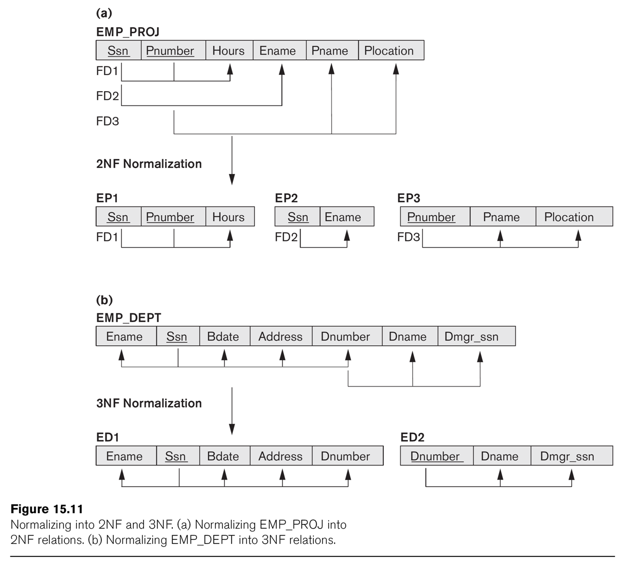
Can we
factor this out?
The LOTS1 relation above (EN fig 15.12) is not 3NF, because of Area ⟶
Price. So we
factor on Area ⟶ Price, dividing into LOTS1A(property_ID,
county,lot_num,area) and
LOTS1B(area,price). Another approach would be to drop price entirely,
if it is in fact proportional
to area, and simply treat it as a computed attribute.
4343
Multiple factoring outcomes
Consider a relation ⟨K1, K2, A, B, C⟩ where K1,K2 is the key and we
have dependencies K1⟶B and B⟶C. If we try to put into 2NF first,
by "factoring out" K1⟶B, we get tables ⟨K1,K2,A,C⟩ and ⟨K1,B⟩; the
dependency B⟶C is no longer expressible in terms of the tables. But if
we start by factoring out B⟶C, we get ⟨K1,K2,A,B⟩ and ⟨B,C⟩; we can now
factor out K1⟶B which yields relations ⟨K1,K2,A⟩, ⟨K1,B⟩ and ⟨B,C⟩; all
functional dependencies have now been transformed into key constraints. Factoring can lose dependencies, or, more
accurately, make them no longer expressible except in terms of the
re-joined tables.
An aid to dealing with this sort of situation is to notice that in
effect we have a three-stage dependency: K1⟶B⟶C. These are often best
addressed by starting with the downstream (B⟶C) dependency.
Boyce-Codd Normal Form
BCNF requires that whenever there is a nontrivial functional dependency
X⟶A, then X is a superkey. It differs from 3NF in that 3NF requires either that X be a superkey or that A be prime (a member of
some key). To put it another way, BCNF bans all nontrivial nonsuperkey
dependencies X⟶A; 3NF makes an exception if A is prime.
As for 3NF, we can use factoring to put a set of tables into BCNF.
However, there is now a serious problem: by factoring out a prime attribute A, we can destroy
an existing key constraint! This is undesireable.
The canonical example of a relation in 3NF but not BCNF is ⟨A, B, C⟩ where we also have
C⟶B. Factoring as above leads to ⟨A, C⟩ and ⟨C, B⟩. We have lost the key
A,B! However, this isn't quite all it appears, because from C⟶B we can conclude A,C⟶B,
and thus that A,C is also a key, and might
be a better choice of key than A,B.
LOTS1A from above was 3NF and BCNF. But now let us suppose that
DeKalb county lots
have sizes <= 1.0 acres, while Fulton county lots have sizes >1.0
acres; this means we now have an
additional dependency FD5: area⟶county. This
violates BCNF, but not 3NF as county is a prime attribute.
If we fix LOTS1A as in Fig 15.13, dividing into LOTS1AX(property_ID,area,lot_num)
and LOTS1AY(area,county),
then we lose the functional
dependency FD2: (county,lot_num)⟶property_ID.

Where has it gone?
This was more than just a random FD; it was a candidate key for LOTS1A.
All databases enforce primary-key constraints. One could use a CHECK
statement to enforce the lost FD2 statement, but this is often a lost
cause.
CHECK (not exists (select ay.county,
ax.lot_num, ax.property_ID, ax2.property_ID
from LOTS1AX ax, LOTS1AX ax2, LOTS1AY ay
where ax.area = ay.area and ax2.area = ay.area
// join condition
and ax.lot_num = ax2.lot_num
and ax.property_ID <> ax2.property_ID))
We might be better off ignoring FD5 here, and just allowing for the
possibility that area does not determine county, or determines it only
"by accident".
Generally, it is good practice to normalize to 3NF, but it is often not
possible to achieve BCNF. Sometimes, in fact, 3NF is too inefficient,
and we re-consolidate for the sake of efficiency two tables factored
apart in the 3NF process.
Fourth Normal Form
Suppose we have tables ⟨X,Y⟩ and ⟨X,Z⟩. If we join on X, we get
⟨X,Y,Z⟩. Now choose a particular value of x, say x0, and consider all
tuples ⟨x0,y,z⟩. If we just look at the y,z part, we get a cross product
Y0×Z0, where Y0={y in Y | ⟨x0,y⟩ is in ⟨X,Y⟩} and Z0={z in Z
| ⟨x0,z⟩ is in ⟨X,Z⟩}. As an example, consider tables
EMP_DEPENDENTS = ⟨ename,depname⟩ and EMP_PROJECTS = ⟨ename,projname⟩:
EMP_DEPENDENTS
ename
|
depname
|
Smith
|
John
|
Smith
|
Anna
|
EMP_PROJECTS
ename
|
projname
|
Smith
|
projX
|
Smith
|
projY
|
Joining gives
ename
|
depname
|
projname
|
Smith
|
John
|
X
|
Smith
|
John
|
Y
|
Smith
|
Anna
|
X
|
Smith
|
Anna
|
Y
|
Fourth normal form attempts to recognize this in reverse, and undo it.
The point is that we have a table ⟨X,Y,Z⟩ (where X, Y, or Z may be a set of attributes), and it turns
out to be possible to decompose it into ⟨X,Y⟩ and ⟨X,Z⟩ so the join is lossless. Furthermore,
neither Y nor Z depend on X, as was the case with our 3NF/BCNF
decompositions.
Specifically, for the "cross product phenomenon" above to occur, we
need to know that if t1 = ⟨x,y1,z1⟩ and t2 = ⟨x,y2,z2⟩ are in ⟨X,Y,Z⟩,
then so are t3 = ⟨x,y1,z2⟩ and t4 = ⟨x,y2,z1⟩. (Note that this is the
same condition as in E&N, 15.6.1, p 533, but stated differently.)
If this is the case, then X is said to multidetermine
Y (and Z). More to the point, it means that if we decompose into ⟨X,Y⟩
and ⟨X,Z⟩ then the join will be lossless.
Are you really supposed even to look
for things like this? Probably not.
Fifth Normal Form
5NF is basically about noticing any other kind of lossless-join
decomposition, and decomposing. But noticing such examples is not easy.
16.4 and the problems of NULLs
"There is no fully satisfactory
relational design theory as yet that includes NULL values"
[When joining], "particular care must
be devoted to watching for potential NULL values in foreign keys"
Unless you have a clear reason for doing otherwise, don't let
foreign-key columns be NULL. Of course, we did just that in the
EMPLOYEE table: we let dno be null to allow for employees not yet
assigned to a department. An alternative would be to create a fictional
department "unassigned", with department number 0. However, we then
have to assign Department 0 a manager, and it has to be a real manager in the EMPLOYEE table.
Ch 17: basics of disks
Databases are often too big to fit everything into main memory, even today,
and disks work differently from memory. Disks are composed of blocks. At the hardware level the
basic unit of the sector
is typically 512 bytes, but the operating system clusters these
together into blocks of size 5K-10K. In the Elder Days applications
would specify their blocksize, but that is now very rare.
A disk looks to the OS like an array of blocks, and any block can be
accessed independently. To access a block, though, we must first move
the read head to the correct track
(seek time) and then wait for the correct block to come around under
the head (rotational latency). Typical mean seek times are ~3-4ms
(roughly proportional to how far the read head has to move, so seeks of
one track over are more like a tenth that). For rotational latency we
must wait on average one-half revolution; at 6000 rpm that is 5ms. 6000
rpm is low nowadays, a reasonable value here is again 3-4 ms and so
accessing a random block can take 6-8ms.
Managing disk data structuresis
all about arranging things so as to minimize the number of
disk-block fetches. This is a very different mind-set from managing
in-memory data structures, where all fetches are equal [ok,
more-or-less equal, for those of you obsessed with cache performance].
When processing a file linearly,
a common technique is read-ahead,
or double-buffering. As the CPU begins to process block N, the IO
subsystem requests block N+1. Hopefully, by the time the CPU finishes
block N, block N+1 will be available. Reading ahead by more than 1
block is also possible (and in fact is common). Unix-based systems
commonly begin sequential read-ahead by several blocks as soon as a
sequential pattern is observed, eg we read 3-4 blocks in succession.
When handling requests from multiple processes, disks usually do not retrieve blocks in FIFO order.
Instead, typically the elevator
algorithm
is used: the disk arm works from the low-numbered track upwards; at
each track, it handles all requests received by that time for blocks on
that track. When there are no requests for higher-numbered tracks, the
head moves back down.
Records can take up a variable amount space in a block; this is annoying, as it
makes finding the kth record on the block more tedious. Still, once the
block is in memory, accessing all the records is quick. It is rare for
blocks to contain more than a hundred records.
BLOBs (binary large objects) are usually not stored within records; the
records instead include a pointer to the BLOB.
File organizations
The simplest file is the heap
file, in which records are stored in order of addition. Insertion is
efficient; search takes linear time. Deletion is also slow, so that
sometimes we just mark space for deletion.
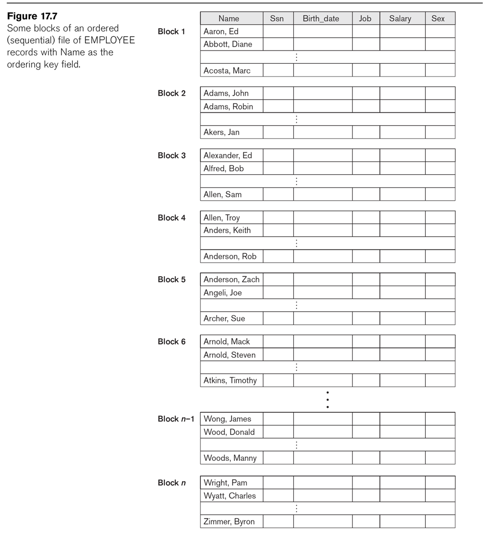
Another format is to keep the records ordered (sorted) by some field, the ordering field.
This is not necessarily a key; for example, we could keep file Employee
ordered by Dno. If the ordering field is a key, we call it the ordering key. Ordered access is now
fast, and search takes log(N) time (where N is the length of the file in blocks
and we are counting only block accesses). Note that the actual
algorithm for binary search is slightly different from the classic
array version: if we have blocks lo
and hi,
and know that the desired value X must, if present, lie between these
two blocks, then we retrieve the block approximately in between, mid. We then check to see one of
these cases:
- X < key of first record on block mid
- X > key of last record on block mid
- X is between the keys, inclusive, and so either the record is on mid or is not found
Note also that the order relation used to order the file need not
actually have any meaning terms of the application! For example,
logically it makes no sense to ask whose SSN is smaller. However,
storing an employee file ordered by SSN makeslookups much faster.
See Fig 17.7
Insertion and deletion are expensive. We can improve insertion by
keeping some unused space at the end of each block for new records (or
the moved-back other records of the block). We can improve deletion by
leaving space at the end (or, sometimes, right in the middle).
Another approach is to maintain a transaction
file:
a sequential file consisting of all additions and deletions.
Periodically we update the master file with all the transactions, in
one pass.
Hashing
Review of internal (main-memory-based) hashing. We have a hash function h that applies to the key values, h = hash(key).
- bucket hashing: the hash table component hashtable[h] contains a pointer to a linked list of records for which hash(key) = h.
- chain hashing: if object Z hashes to value h, we try to put Z at hashtable[h]. If that's full, we try hashtable[h+1], etc.
For disk files, we typically use full blocks as buckets. However,
these
will often be larger than needed. As a result, it pays to consider hash
functions that do not generate too many different values; a common
approach is to consider hash(key) mod N, for a smallish N (sometimes
though not universally a prime number).
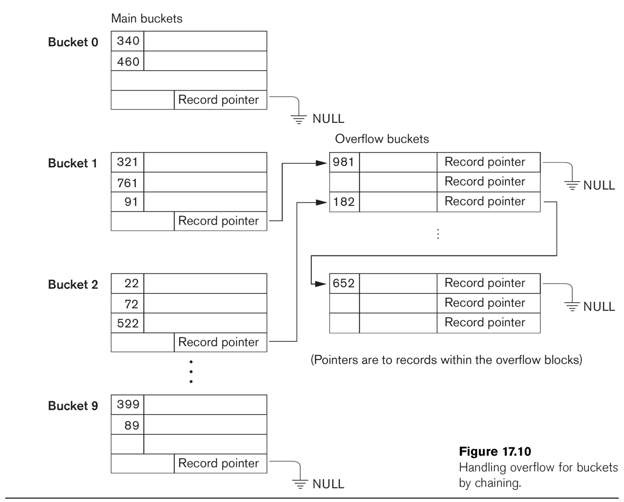
Given a record, we will compute h = hash(key). We also provide a
single-block map ⟨hash,block⟩ of hash values to block
addresses (in effect corresponding to hashtable[]). Fig 17.9 shows the
basic strategy. More detail on the buckets is provided in Fig 17.10,
which also shows some overflow buckets. Note that Bucket 1 and Bucket 2
share
an overflow bucket; we also can (and do) manipulate the ⟨hash,block⟩
structure so that two buckets share a block (by entering ⟨hash1,block1⟩
and ⟨hash2,block2⟩ where block1 = block2). When
a single bucket approaches two blocks, it can be given its own overflow
block.
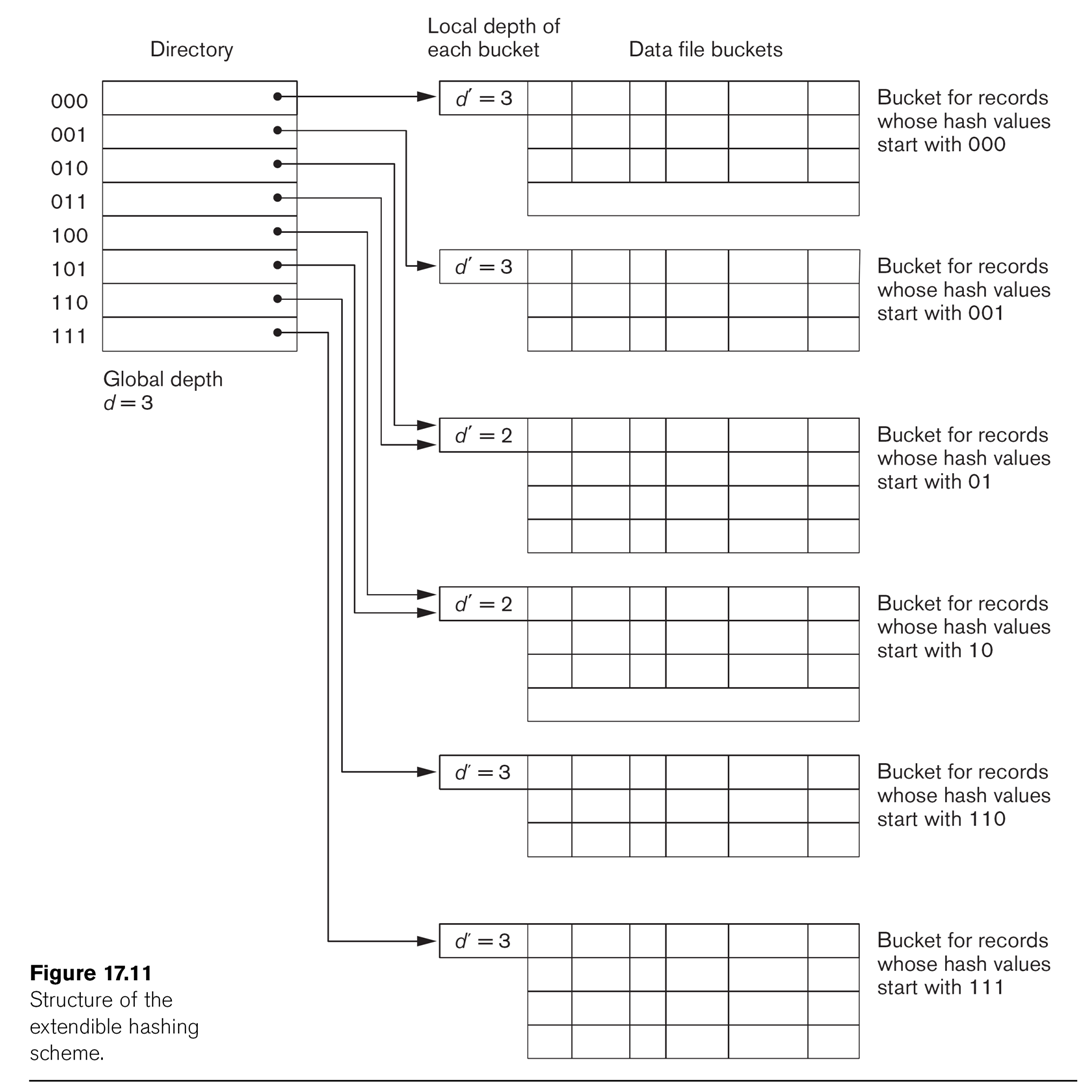
Extendible Hashing
This technique manages buckets more efficiently. We hash on the first d bits of the hash values; d is
called the global depth. We
keep a directory of all 2d possible values for these d bits,
each with a pointer to a bucket block. Sometimes, two neighboring
buckets are consolidated
in the directory; for example, if d=3, hash prefix values 010 and 011
might point to the same block. That block thus has a reduced local depth of 2.
As we fill blocks, we need to create new ones. If a block with a
reduced local depth overflows, we split it into two blocks with a
greater depth (still ≤ d). If a block with local depth d overflows, we
need to make some global changes: we increment d by 1, double the directory size, and double up all
existing blocks except for the one causing the overflow.
See Fig 17.11.
Extendible hashing grew out of dynamic
hashing,
in which we keep a tree structure of hashcode bits, stopping when we
have few enough values that they will all fit into one block.
Ch 18: indexing
It is common for databases to provide indexes for files. An index can be on either a key field or a non-key field; in the latter case it is called a clustering index. The index can either be on a field by which the file is sorted or not. An index can have an entry for every record, in which case it is called dense; if not, it is called sparse.
An index on a nonkey field is always considered sparse, since if every
record had a unique value for the field then it would in fact be a key
after all.
A file can have multiple indexes, but the file itself can be structured
only for one index. We'll start with that case. The simplest file
structuring for the purpose of indexing is simply to keep the file
sorted on the attribute being indexed; this allows binary search. For a
while, we will also keep restrict attention to single-level indexes.
Primary Index
A primary index is an index on the primary key of a sorted file (note that an index on the primary key, if the file is not maintained as sorted on that primary key, is thus not a "primary index"!). The
index consists of an ordered list of pairs ⟨k,p⟩, where k is the
first key value to appear in the block pointed to by p (this first
record of each block is sometimes called the anchor record).
To find a value k in the file, we find consecutive ⟨k1,p⟩ and ⟨k2,p+1⟩ where k1≤k<k2; in that case, the record with key k
must be on block p. This is an example of a sparse index. A primary index is usually much smaller than the file itself. See Fig 18.1.
Example 1 on EN6 p 635: 30,000 records, 10 per block, for 3000
blocks. Direct binary search takes 12 block accesses. The index entries
are 9+6 bytes long, so 1024/15 = 68 fit per 1024-byte block. The index has 3000/68 = 45
blocks; binary search requires 6 block accesses, plus one more for the
actual data block itself.
Clustering index
We can also imagine the file is ordered on a nonkey field (think Employee.dno). In this case we create a clustering index.
The index structure is the same as before, except now the block pointer
points to the first block that contains any records with that value;
see Fig 18.2.
Clustering indexes are of necessity sparse. However, it is not
necessary to include in the index every value of the attribute; we only
need to include in the index the attribute values that appear first in
each block. But there's a tradeoff; if we skip some index values then
we likely will want an index entry for every block; for a non-key index
this may mean many more entries than an index entry for every distinct
value. In Fig 18.2, we have an entry for every distinct value; we
could remove the entries for Dept_number=2 and Dept_number=4.
Another approach to clustering indexes may be seen in Fig 18.3, in
which blocks do not contain records with different cluster values. Note that this is again a method of organizing the file for the purpose of the index.
Secondary Indexes
Now suppose we want to create an index for Employee by (fname, lname),
assumed for the moment to be a secondary key. The record file itself is
ordered by Ssn. An index on a secondary key
will necessarily be dense, as the file won't be ordered by the secondary key; we cannot use block anchors. A common
arrangement is simply to have the index list ⟨key,block⟩ pairs
for every key value appearing; if there are N records in the file then
there will be N in the index and the only savings is that the index
records are smaller. See Fig 18.4. If B is the number of blocks in the
original file, and BI is the number of blocks in the index, then BI ≤B,
but not by much, and log(BI) ≃ log(B), the search time. But note that
unindexed search is linear now, because the file is not ordered on the secondary key.
Example 2, EN6, p 640: 30,000 records, 10 per block. Without an
index, searching takes 1500 blocks on average. Blocks in the index hold
68 records, as before, so the index needs 30,000/68 = 442 blocks;
log2(442) ≃ 9.
Secondary indexes can also be created on nonkey
fields. We can create dense indexes as above, but now with multiple
entries for the indexed attribute, one for each
record (Option 1 in EN6 p 640). A second approach (option 2 in EN6 p
640) is to have the index consist of a single entry for each value of
the indexed attribute, followed by a list of record pointers. The third option, perhaps the most common, is for each index entry to point to blocks of record
pointers, as in Fig 18.5.
Hashing
Hashing can be used to create a form of index, even if we do not structure the file that way. Fig 18.15 illustrates an example. We can
use hashing with equality comparisons, but not order comparisons, which
is to say hashing can help us find a record with ssn=123456789, but
not records with salary between 40000 and 50000. Hash indexes are, in
theory, a good index for joins. Consider the join
select e.lname, w.pno, w.hours from employee e, works_on w where e.ssn = w.essn;
We might choose each record e from employee, and want to find all
records in works_on with e.ssn = w.essn. A hash index for works_on, on
the field essn, can be useful here. Note this can work even though
works_on.essn is not a key field.
There is one problem: we are likely to be retrieiving blocks of
works_on in semi-random order, which means one disk access for each
record. However, this is still faster than some alternatives.
Multilevel indexes
Perhaps our primary sorted index grows so large that we'd like an index for it. At that point we're creating a multi-level index. To create the ISAM index, we start with the primary
index, with an index entry for the anchor record of each block, or a secondary index, with an entry for each record. Call
this the base level, or first level, of the index. We now create a second level index containing an index entry for the anchor record of each block of the first-level index. See Fig 18.6. This is called an indexed sequential file, or an ISAM file.
This technique works as well on secondary keys, except that the first level is now much larger.
What is involved in inserting
new records into an ISAM structure? The first-level index has to be
"pushed down"; unless we have left space ahead of time, most blocks
will need to be restructured. Then the second and higher-level indexes
will also need to be rebuilt, as anchor records have changed.
Example: we have two records per block, and the first level is
Data file: 1 2 3
5 7 9 20
1st-level index: 1 3 7 20
What happens when we insert 8? 4? 6?
What happens when we "push up a level", that is, add an entry that forces us to have one higher level of index?
EN6 Example 3 (p 644): 30,000 records and can fit 68 index entries per block. The first-level index is 30,000/68 = 442 blocks,
second-level index is 442/68 = 7 blocks; third-level index is 1 block.
B-trees (Bayer trees)
Consider a binary search tree for the moment. We decide which of the two leaf nodes to pursue at each point based on comparison.
We can just as easily build N-ary search trees, with N leaf nodes and N-1 values stored in the node. Consider the ternary example for a moment.
Next, note that we can have a different N at each node!
Bayer trees: let's have a max of 4 data items per node.
1 4 8 9 20 22 25 28
How can we add nodes so as to remain balanced? We also want to minimize partial blocks. A B-tree of order p means that each block has at most p tree pointers, and p-1 key values. In addition, all but the top node has at least (p-1)/2 key values.
"push-up" algorithm: we add a new value to a leaf block. If there is room, we are done. If not, we split the block and push up the middle value to the parent block.
The parent block may now also have to be split.
B+ trees: slight technical improvement where we replicate all the key values on the bottom level.
Databases all support some mechanism of creating indexes, of specific types. For example, MySQL allows
CREATE INDEX indexname ON employee(ssn) USING BTREE; // or USING HASH
Example query (E&N6, p 660):
select e.fname, e.lname from employee e where e.dno = 4 and e.age=59;
If we have an index on dno, then access that cluster using the index and search for age.
If we have an index on age, we can use that.
If we have an index on (dno, age), we have a single lookup! But we also have expensive indexes to maintain.
Indexes can be ordered or not; ordered indexes help us find employees
with e.age >= 59. Ordered and nonordered indexes both support
lookup; ordered indexes also in effect support return of an iterator yielding all DB records starting at the specified point. BTREE and ISAM indexes are ordered; HASH indexes are not.
Basics of forms
A form is enclosed between <form method="post" action="program">
and </form> tags. The usual value for action is "", meaning to
re-invoke the same program (in our case, a php program), but now with posted data values.
Inside the form you can have input items, of the form <input type="input-type" ... >. Input items can be
- text (one-line text boxes)
- button (clickable buttons)
- radio (radio buttons)
- checkbox (checkboxes)
- select: menus with options
- select ... multiple: allows selecting several items simultaneously
- textarea (scrolling text boxes)
- submit (submit buttons, semantically different from ordinary buttons)
- more
Here's a big form. You can see it in action at form1.html.
<form action="form1.cgi" method="get" enctype="multipart/form-data">
<input type = "button" value="click me!" name="b1">
<input type = "button" value="me too!" name="b2">
<p> Are we having fun yet?
<center>
<input type="radio" name="fun" value = "yes">Yep!
<input type="radio" name="fun" value = "no">Nope!
<input type="radio" name="fun" value = "maybe" CHECKED>I dunno!
</center>
<p><b>Why are you doing this?</b>
<input type = "checkbox" name="cbox" value="credit" CHECKED>For course credit
<input type = "checkbox" name="cbox" value="money" CHECKED>For the money!
<br>
<p><b>Who are you?</b>
<input type = "text" name="name1" value="I dunno" size=20>
<p>Now for a menu:
<p>
<select size = 1 name="menu1">
<option> first item
<option> second item
<option> number 3!
<option> fourth
<option> last
</select>
<p> now with size=4</p>
<select size = 4 name="menu2" multiple>
<option> first item
<option> second item
<option> number 3!
<option> fourth
<option> last
</select>
<p>Here's a text box</p>
<textarea name="mybox" rows=5 cols = 30>
This message will be in the box. It's plain text, <b>not</b> html!
I'm going to make it long enough that a scrollbar appears,
through the miracle of cut-and-paste.
I'm going to make it long enough that a scrollbar appears,
through the miracle of cut-and-paste.
</textarea>
<p>
<input type="submit">
</form>
Understand the form action, and the idea tha tone page can have multiple <form ...> ... </form> objects.