Comp 353/453: Database Programming, Corboy L08, 4:15 Mondays

Week 12, Apr 15


Ch 18: indexing

It is common for databases to provide indexes for files. An index can be on either a key field or a non-key field; in the latter case it is called a clustering index. The index can either be on a field by which the file is sorted or not. An index can have an entry for every record, in which case it is called dense; if not, it is called sparse. An index on a nonkey field is always considered sparse, since if every record had a unique value for the field then it would in fact be a key after all.

Example 1 on EN6 p 635: 30,000 records, 10 per block, for 3000 blocks. Direct binary search takes 12 block accesses. The index entries are 9+6 bytes long, so 1024/15 = 68 fit per 1024-byte block. The index has 3000/68 = 45 blocks; binary search requires 6 block accesses, plus one more for the actual data block itself. There is also an excellent chance that the entire 45-block index will fit in RAM.

Primary Index

A primary index is an index on the primary key of a sorted file (note that an index on the primary key, if the file is not maintained as sorted on that primary key, is thus not a "primary index"!). The index consists of an ordered list of pairs ⟨k,p⟩, where k is the first key value to appear in the block pointed to by p (this first record of each block is sometimes called the anchor record). To find a value k in the file, we find consecutive ⟨k1,p⟩ and ⟨k2,p+1⟩ where k1≤k<k2; in that case, the record with key k must be on block p. This is an example of a sparse index. A primary index is usually much smaller than the file itself. See Fig 18.1.

Example 1 on EN6 p 635: 30,000 records, 10 per block, for 3000 blocks. Direct binary search takes 12 block accesses. The index entries are 9+6 bytes long, so 1024/15 = 68 fit per 1024-byte block. The index has 3000/68 = 45 blocks; binary search requires 6 block accesses, plus one more for the actual data block itself.

Clustering index

We can also imagine the file is ordered on a nonkey field (think Employee.dno). In this case we create a clustering index. The index structure is the same as before, except now the block pointer points to the first block that contains any records with that value; see Fig 18.2. Clustering indexes are of necessity sparse. However, it is not necessary to include in the index every value of the attribute; we only need to include in the index the attribute values that appear first in each block. But there's a tradeoff; if we skip some index values then we likely will want an index entry for every block; for a non-key index this may mean many more entries than an index entry for every distinct value.  In Fig 18.2, we have an entry for every distinct value; we could remove the entries for Dept_number=2 and Dept_number=4.

Another approach to clustering indexes may be seen in Fig 18.3, in which blocks do not contain records with different cluster values. Note that this is again a method of organizing the file for the purpose of the index.

Ordering a file by a nonkey field may sound unlikely. However, it may be quite useful in cases where the file has a multi-attribute key. For example, we might keep the works_on file ordered by essn; the essn alone is not a key. This would allow easy lookup of any employee's projects. We might in fact keep the file ordered lexicographically by the full key, ⟨essn,pno⟩, in which case the file would be automatically ordered by essn alone, and we could create a clustering index on essn alone. Yet another example of a plausible clustering index is the invoice_item file we considered previously. The key is ⟨invoice_num, partnum⟩. Keeping the file ordered first by invoice_num and second by partnum would allow a clustering index on invoice_num alone, which is likely to be something we frequently need to do. (This example is in some sense the same as the works_on example.)

Secondary Indexes

Now suppose we want to create an index for Employee by (fname, lname), assumed for the moment to be a secondary key. The record file itself is ordered by SSN. An index on a secondary key will necessarily be dense, as the file won't be ordered by the secondary key; we cannot use block anchors. A common arrangement is simply to have the index list ⟨key,block⟩ pairs for every key value appearing; if there are N records in the file then there will be N in the index and the only savings is that the index records are smaller. See Fig 18.4. If B is the number of blocks in the original file, and BI is the number of blocks in the index, then BI ≤B, but not by much, and log(BI) ≃ log(B), the search time. But note that unindexed search is linear now, because the file is not ordered on the secondary key.

Example 2, EN6, p 640: 30,000 records, 10 per block. Without an index, searching takes 3,000/2 = 1500 blocks on average. Blocks in the index hold 68 records, as before, so the index needs 30,000/68 = 442 blocks; log2(442) ≃ 9.

Secondary indexes can also be created on nonkey fields. We can create dense indexes as above, but now with multiple entries for the indexed attribute, one for each record (Option 1 in EN6 p 640). A second approach (option 2 in EN6 p 640) is to have the index consist of a single entry for each value of the indexed attribute, followed by a list of record pointers. The third option, perhaps the most common, is for each index entry to point to blocks of record pointers, as in Fig 18.5.

index on file ordered by

example
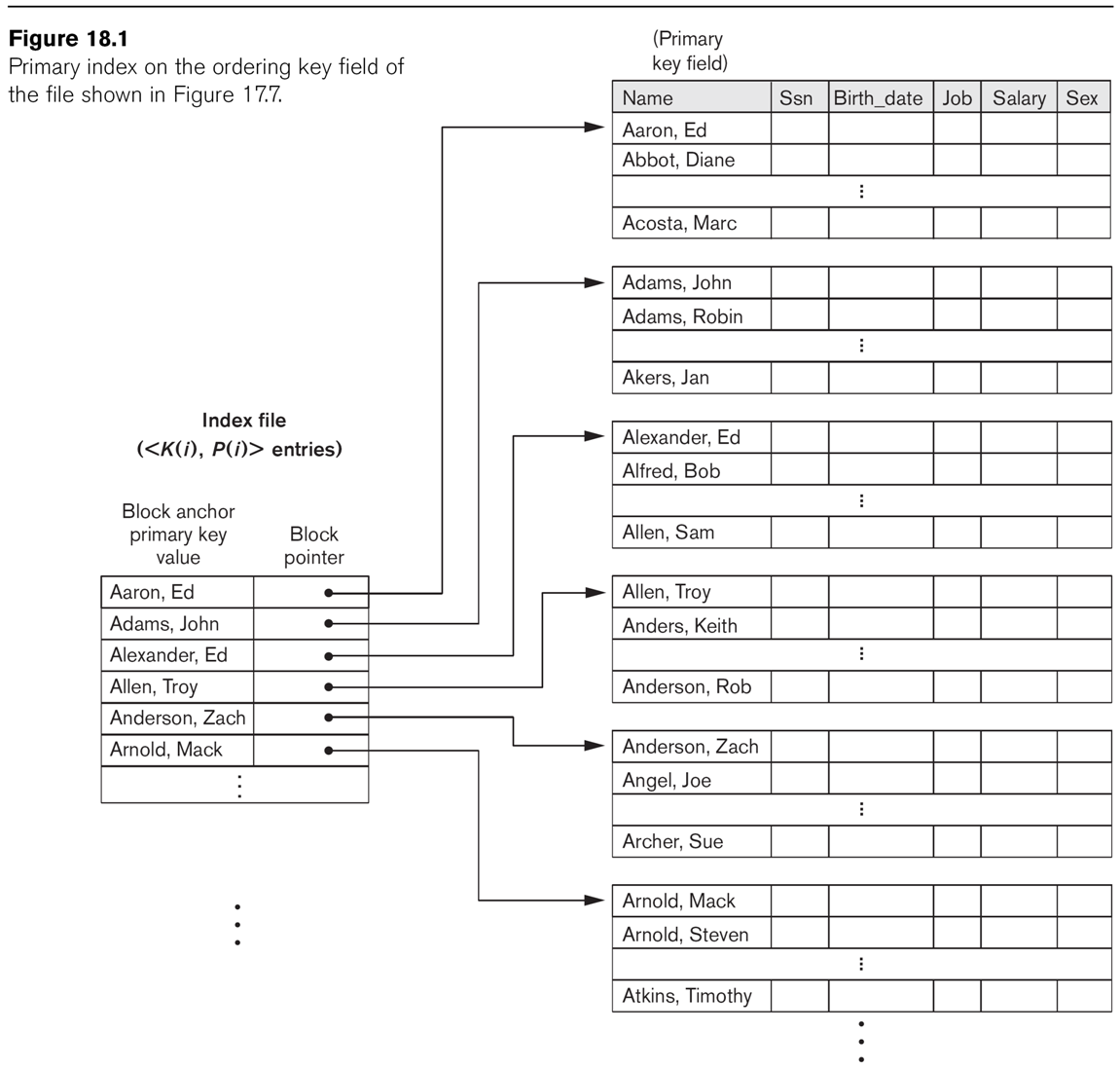
key value
(primary index)
that key value sparse
fig 18.1
key value
(secondary key?)
something else dense
fig 18.4
nonkey value
(clustering)
that nonkey value sparse
figs 18.2, 18.3
nonkey value
(clustering)
something else sparse
fig 18.5

Hashing

Hashing can be used to create a form of index, even if we do not structure the file that way. Fig 18.15 illustrates an example; the hash function in this example is the final digit of the sum of the digits of the employee number.

Hashing with equality comparisons, but not order comparisons, which is to say hashing can help us find a record with ssn=123456789, but not records with salary between 40000 and 50000. Hash indexes are, in theory, a good index for joins. Consider the join

    select e.lname, w.pno, w.hours from employee e, works_on w where e.ssn = w.essn;

We might choose each record e from employee, and want to find all records in works_on with e.ssn = w.essn. A hash index for works_on, on the field essn, can be useful here. Note this can work even though works_on.essn is not a key field.

There is one problem: we are likely to be retrieving blocks of works_on in semi-random order, which means one disk access for each record. However, this is still faster than some alternatives.

Multilevel indexes

Perhaps our primary sorted index grows so large that we'd like an index for it. At that point we're creating a multi-level index. To create this kind of index, we start with the primary index, with an index entry for the anchor record of each block, or a secondary index, with an entry for each record. Call this the base level, or first level, of the index. We now create a second level index containing an index entry for the anchor record of each block of the first-level index. See Fig 18.6. We keep adding levels until we get to a top-level index that fits in a single block. This is called an indexed sequential file, or an ISAM (Indexed Sequential Access Method) file.

This technique works as well on secondary keys, except that the first level is now much larger.

What is involved in inserting new records into an ISAM structure? The first-level index has to be "pushed down"; unless we have left space ahead of time, most blocks will need to be restructured. Then the second and higher-level indexes will also need to be rebuilt, as anchor records have changed.

Example: we have two records per block, and the first level is

Data file:          1 2        3 5    7  9      20
1st-level index:    1 3       7 20
2nd-level index:    1 7


What happens when we insert 8? 4? 6?

What happens when we "push up a level", that is, add an entry that forces us to have one higher level of index?

EN6 Example 3 (p 644): 30,000 records and can fit 68 index entries per block. The first-level index is 30,000/68 = 442 blocks, second-level index is 442/68 = 7 blocks; third-level index is 1 block.

B-trees (Bayer trees)

Consider a binary search tree for the moment. We decide which of the two leaf nodes to pursue at each point based on comparison.

We can just as easily build N-ary search trees, with N leaf nodes and N-1 values stored in the node. Consider the ternary example for a moment.

Next, note that we can have a different N at each node!

Bayer trees: let's have a max of 4 data items per node. Here is a tree with a single value in its root node and two (four-value_ leaf nodes:


              15
          /        \
1 4  8  9            20 22 25 28

Here's a tree with two values in its root node, and three leaf nodes. One of the leaf nodes is not "full". (This tree cannot be reached by inserting values into the tree above.)

                 15    30
             /      |      \
           /        |        \
1  4  8  9     20 22 25 28     31 37 42

How can we add nodes so as to remain balanced? We also want to minimize partial blocks. A B-tree of order p means that each block has at most p tree pointers, and p-1 key values. In addition, all but the top node has at least (p-1)/2 key values.

"Push-up" algorithm: To add a new value, we start by adding it to a leaf block. If there is room, we are done. If not, we split the block and push up the middle value to the parent block.

The parent block may now also have to be split.

The tree only grows in height when the push-up process bumps up a new root block; the tree remains balanced.

There is a nice java-applet animation of B-tree insertion at http://slady.net/java/bt/view.php?w=800&h=600.

B+ trees: slight technical improvement where we replicate all the key values on the bottom level.


Databases all support some mechanism of creating indexes, of specific types. For example, MySQL allows
   
   
CREATE INDEX indexname ON employee(ssn) USING BTREE;    // or USING HASH

Example query (E&N6, p 660):
    select e.fname, e.lname from employee e where e.dno = 4 and e.age=59;

If we have an index on dno, then access that cluster using the index and search for age.
If we have an index on age, we can use that.
If we have an index on (dno, age), we have a single lookup! But we also have expensive indexes to maintain.

Indexes can be ordered or not; ordered indexes help us find employees with e.age >= 59. Ordered and nonordered indexes both support lookup; ordered indexes also in effect support return of an iterator yielding all DB records starting at the specified point. BTREE and ISAM indexes are ordered; HASH indexes are not.


Indexes v File Organization

What's the difference between creating a hashed file organization and a hashed index? Or a B-tree file organization versus a B-tree index? An index needs to stand alone, and allow finding any given record; a file-organization method generally allows us to retrieve blocks of records at a time.

A B-tree index technically has to be a B+-tree, as a B-tree includes file blocks at interior levels. The usual B/B+ tree also includes many related records in single leaf blocks, but that is straightforward to give up (at the cost of much less efficient traversal).


Query processing

First, note it is relatively easy to sort records. Typically we will use merge-sort, where we subdivide into blocks small enough to fit into memory. We sort those with, say, quicksort. We then make passes until each pair of consecutive blocks is merged.

Select

Some examples
  1. select * from employee e where e.ssn = '123456789'
  2. select * from department where dnumber >=5
  3. select * from employee where dno = 5
  4. select * from employee where dno = 5 and salary > 30000 and sex = 'F'
  5. select * from works_on where essn='123456789' and pno=10
Methods of implementation:

Linear search: we read each disk block once.
Binary search: this is an option if the selection condition is an equality test on a key attribute, and the file is ordered by that attribute.
Primary index: same requirement as above, plus we need an index
Hash search: equality comparison on any attribute for which we have a hash index (need not be a key attribute)
Primary index and ordered comparison: use the index to find all departments with dnumber > 5
Clustered index (includes hash indexes)
B-tree index

If we are searching for "dno=5 AND salary=4000" we can use an index for either attribute, or a composite index if one exists.

In general, we'd like to choose the condition with the fewest results, and then continue with the remaining conditions.

For OR conditions, we just have to search for each.

For the examples above, here are some notes on which select implementation is likely to be most efficient.

  1. For this query, an index on employee.ssn is likely to be fastest. Any index will do.
  2. For this query, the range comparison (dnumber >= 5) means that unless we have an "ordered" index (that is, a B-tree or a "primary index") we might find linear search hard to beat. Note that this is a search by key attribute.
  3. For this query, an index on dno would be a clustering index as in figs 18.2, 18.3 and 18.5. This index could be used, and if the employee file were ordered by dno then the minimum number of blocks would need to be retrieved. But this is unlikely; and that in turn means that using the index might still involve retrieving nearly ever block of the employee file (for example, if almost every block contained at least one member of department 5). Linear search in such a case would be hard to beat.
  4. In this case we have three selection criteria. We are best off applying the most selective criterion first. Unless we know something about the distribution of salaries, we can assume that "salary>30000" is about 50% likely to be true; the same might be true for "sex = 'F'". We are best off starting with dno=5, and then searching only those records for the ones that also satisfy the other two criteria.
  5. Note that the primary key to works_on is the pair (essn,pno). If we have a primary-key index, we can simply look this up. But if we keep the file ordered by essn, and with an index on essn, then we can also use that to find the answer; most employees work on only a small number of projects so works_on.lookup(essn) will be small.

Joins

Mostly we focus on equijoins:
  1. select * from employee e, department d where e.dno = d.dnumber
  2. select * from department d, employee e where d.mgr_ssn = e.ssn
These joins are quite different. In each case we are joining a key in one table (underlined) to a foreign key in another, but it is likely that the employee table is much larger than the department table. In the first example, the number of records in the join will be (about) the size of the employee table (large); in the second example the number of records in the join will be (about) the size of the department table, much smaller.

We will consider four methods of implementation.

Numeric assumptions for the four methods (Book example, EN6 p 690-693): Suppose we have 6,000 employee records in 2,000 blocks, and 50 departments in 10 blocks. We have indexes on both tables. The employee.ssn index takes 4 accesses, and the dept.dnumber index takes 2.

1. Nested-loop join: this is where we think of a for-loop:

    for (e in employee) {
       for (d in department) {
          if (e.dno = d.dnumber) print(e,d);
       }
    }

The time needed here is NM, where N is the size of employee and M is the size of department; loosely speaking, we might say this is quadratic. If we go through the employee table record by record, that amounts to 2,000 block accesses. For each employee record the loop above would go through all 10 blocks of departments; that's 6,000 × 10 = 60,000 blocks. Doing it the other way, we go through 10 blocks of departments, and, for each department record, we search 2,000 blocks of employees for 50×2,000 = 100,000 block accesses. In other words, the complexity is not symmetric!

However, note that we can also do this join block-by-block on both files:
Done this way, the number of block accesses is 2,000 × 10 = 20,000 blocks, or, in general, NM, where N and M are now the sizes of the respective tables in blocks.

Performance improves rapidly if we can keep the smaller table entirely in memory: we then need only 2,010 block accesses! (The EN6 analysis makes some additional assumptions about having spare buffer blocks to work with.)


2. Index join: if we have an index on one of the attributes, we can use it:

    for (e in employee) {
       d = lookup(department, e.ssn);
       if (d != null) print(e,d);
    }

Note that any index will do, but that this may involve retrieving several disk blocks for each e and will almost certainly involve retrieving at least one disk block (from department) for every e in employee. It may or may not be better than Method 1.

Consider the first query above. Suppose we have a primary index on department.dno that allows us to retrieve a given department in 2 accesses. Then we go through 6,000 employees and retrieve the department of each; that's 6,000×2 = 12,000 block accesses.

Now consider the second query, and suppose we can find a given employee in 4 accesses. Then we go through 50 × 4 = 200 block accesses (for every department d, we look up d.mgr_ssn in table employee). Of course, as we noted at the beginning, the final result of the second query is a much smaller table.


3. Sort-merge join: we sort both files on the attribute in question, and then do a join-merge. This takes a single linear pass, of size the number of blocks in the two files put together file. This is most efficient if the files are already sorted, but note that it's still faster than 1 (and possibly faster than 2) if we have to sort the files. Assume both tables are sorted by their primary key, and assume we can sort in with N log(N) block accesses, where N is the number of blocks in the file. Then query 1 requires us to sort table employee in time 2,000×11 = 22,000; the actual merge time is much smaller. Query 2 requires us to sort table department in time 10×4 = 40; the merge then takes ~2,000 blocks for the employee table.

4. Partition-hash join: Let the relations (record sets) be R and S. We partition R into disjoint sets Ri = {r ∈ R | hash(r) = i}, and S into Si = {s∈S | hash(s) = i}. Now we note that the join R ⋈ S is simply the disjoint union of the Ri ⋈ Si. In most cases, either Ri or Si will be small enough to fit in memory.

A good hash function helps; we want the buckets to be relatively uniform. We won't get that, but we should hope for Poisson distribution. With N things in K buckets, we expect an average of a=N/K per bucket. The probability of i things is aie-a/i! and the expected number of i-sized buckets is about N*aie-a/i!.


The join selection factor is the fraction of records that will participate in the join. In query 2 above,

    select * from department d, employee e where d.mgr_ssn = e.ssn

all departments will be involved in the join, but almost no employees. So we'd rather go through the departments, looking up managing employees, rather than the other way around.

In the most common case of joins, the join field is a foreign key in one file and a primary key in the other. Suppose we keep all files sorted by their primary key. Then for any join of this type, we can traverse the primary-key file block by block; for each primary-key value we need to do a lookup of the FK attribute in the other file. This would be method 2 above; note that we're making no use of the primary index.


Query optimization

As with compilers, the word "optimization" is used loosely.

A major rule is to apply select/project before joins, and in general do operations first that have greatest potential for reducing the size of the number of records.

Query tree: See fig 19.4.

Select lname from employee e, works_on w, project p
where e.ssn = w.essn and w.pno = p.pnumber and p.pname = 'Aquarius';

See fig 19.5, but note that doing cross-products was never on the agenda. However, it still does help to do the second join first.

Some heuristic rules: