Database week 10

Comp 353/453: Database Programming, Corboy L08, 4:15 Mondays

Week 10, Apr 1

Problem with member---reserves---boat problem on exam:

Reserves is not actually a relationship set: the pair (member, boat) does not determine the relationship. See the notes for Invoice under week 6; the boat-reservation relationship is really best thought of as ternary.

Design guidelines

Review the four guidelines from week 9.
Problem: what do we have to do to meet these guidelines?

Functional Dependencies and Normalization

A functional dependency is a kind of semantic constraint. If X and Y are sets of attributes (column names) in a relation, a functional dependency X⟶Y means that if two records have equal values for X attributes, then they also have equal values for Y.

For example, if X is a set including the key attributes, then X⟶{all attributes}.

Like key constraints, FD constraints are not based on specific sets of records. For example, in the US, we have {zipcode}⟶{city}, but we no longer have {zipcode}⟶{areacode}.

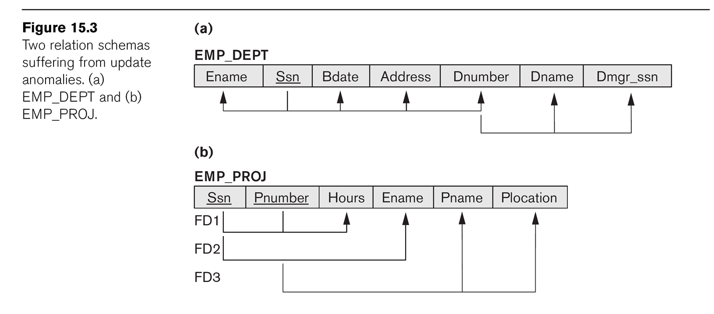
In the earlier EMP_PROJ, we have FDs
    Ssn ⟶ Ename
    Pnumber ⟶ Pname, Plocation
    {Ssn, Pnumber} ⟶ Hours

In EMP_DEPT we have FDs
    Ssn ⟶ Ename, Bdate, Address, Dnumber
    Dnumber ⟶ Dname, Dmgr_ssn

Sometimes FDs are a problem, and we might think that just discreetly removing them would be the best solution. But they often represent important business rules; we can't really do that either. At the very least, if we don't "normalize away" a dependency we run the risk that data can be entered so as to make the dependency fail.

diagram for EMP_PROJ, EMP_DEPT

A superkey (or key superset) of a relation schema is a set of attributes S so that no two tuples of the relationship can have the same values on S. A key is thus a minimal superkey: it is a superkey with no extraneous attributes that can be removed. For example, {Ssn, Dno} is a superkey for EMPLOYEE, but Dno doesn't matter (and in fact contains little information); the key is {Ssn}.

Note that, as with FDs, superkeys are related to the sematics of the relationships, not to particular data in the tables.

Relations can have multiple keys, in which case each is called a candidate key. For example, in table DEPARTMENT, both {dnumber} and {dname} are candidate keys. For arbitrary performance-related reasons we designated one of these the primary key; other candidate keys are known as secondary keys.

A prime attribute is an attribute (ie column name) that belongs to some candidate key. A nonprime attribute is not part of any key. For DEPARTMENT, the prime attributes are dname and dnumber; the nonprime are mgr_ssn and mgr_start.

A dependency X⟶A is full if the dependency fails for every proper subset X' of X; the dependency is partial if not, ie if there is a proper subset X' of X such that X'⟶A.

Normal Forms and Normalization

Normal Forms are rules for well-behaved relations. Normalization is the process of converting poorly behaved relations to better behaved ones.

First Normal Form

First Normal Form (1NF) means that a relation has no composite attributes or multivalued attributes. Note that dealing with the multi-valued location attribute of DEPARTMENT meant that we had to create a new table LOCATIONS. Composite attributes were handled by making each of their components a separate attribute.

Alternative ways for dealing with the multivalued location attribute would be making ⟨dnumber, location⟩ the primary key, or supplying a fixed number of location columns loc1, loc2, loc3, loc4. For the latter approach, we must know in advance how many locations we will need; this method also introduces NULL values.

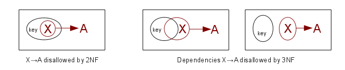
Second Normal Form

Second Normal Form (2NF) means that, if K represents the set of attributes making up the primary key, every nonprime attribute A (that is an attribute not a member of any key) is functionally dependent on K (ie K⟶A), but that this fails for any proper subset of K (no proper subset of K functionally determines A).

Note that if a relation has a single-attribute primary key, as does EMP_DEPT, then 2NF is automatic. (Actually, the general definition of 2NF requires this for every candidate key; a relation with a single-attribute primary key but with some multiple-attribute other key would still have to be checked for 2NF.)

We say that X⟶Y is a full functional dependency if for every proper subset X' of X, X' does not functionally determine Y. Thus, 2NF means that for every nonprime attribute A, the dependency K⟶A is full: no nonprime attribute depends on less than the full key.

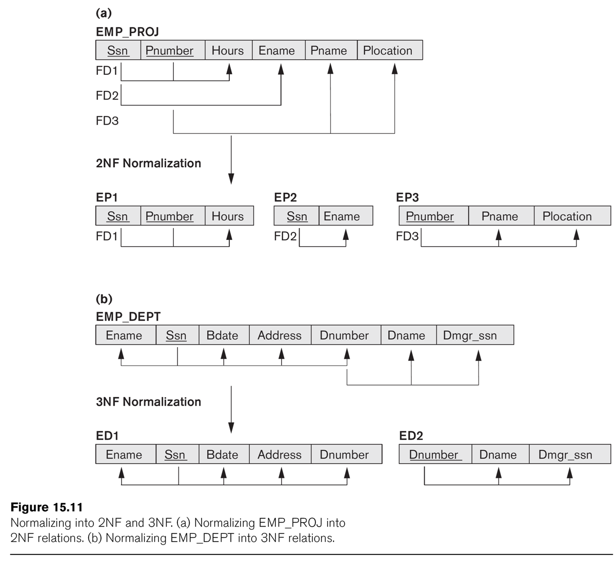
In the earlier EMP_PROJ relationship, the primary key K is {Ssn, Pnumber}. 2NF fails because {Ssn}⟶Ename, and {Pnumber}⟶Pname, {Pnumber}⟶Plocation.

To put a table in 2NF, decompose it into sets of attributes which all have a common full dependency on some subset K' of K. For EMP_PROJ, this becomes:
    ⟨Ssn, Pnumber, Hours⟩
    ⟨Ssn, Ename⟩
    ⟨Pnumber, Pname, Plocation⟩
Note that Hours is the only attribute with a full FD on {Ssn,Pnumber}.

The table EMP_DEPT is in 2NF.

Note that we might have a table ⟨K1, K2, K3, A1, A2, A3⟩, where
    {K1,K2,K3}⟶A1 is full
    {K1,K2}⟶A2 is full (neither K1 nor K2 alone determines A2)
    {K2,K3}⟶A2 is full
    {K1,K3}⟶A3 is full
    {K2,K3}⟶A3 is full

The decomposition could be

    ⟨K1, K2, K3, A1⟩
    ⟨K1, K2, A2⟩
    ⟨K1, K3, A3⟩

or it could be

    ⟨K1, K2, K3, A1⟩
    ⟨K2, K3, A2, A3⟩

Remember, dependency constraints can be arbitrary! Dependency constraints are often best thought of as "externally imposed rules"; they come out of the user-input-and-requirements phase of the DB process. Trying to pretend that there is not a dependency constraint is sometimes a bad idea.

Consider the LOTS example of Fig 15.12.
dependency diagram

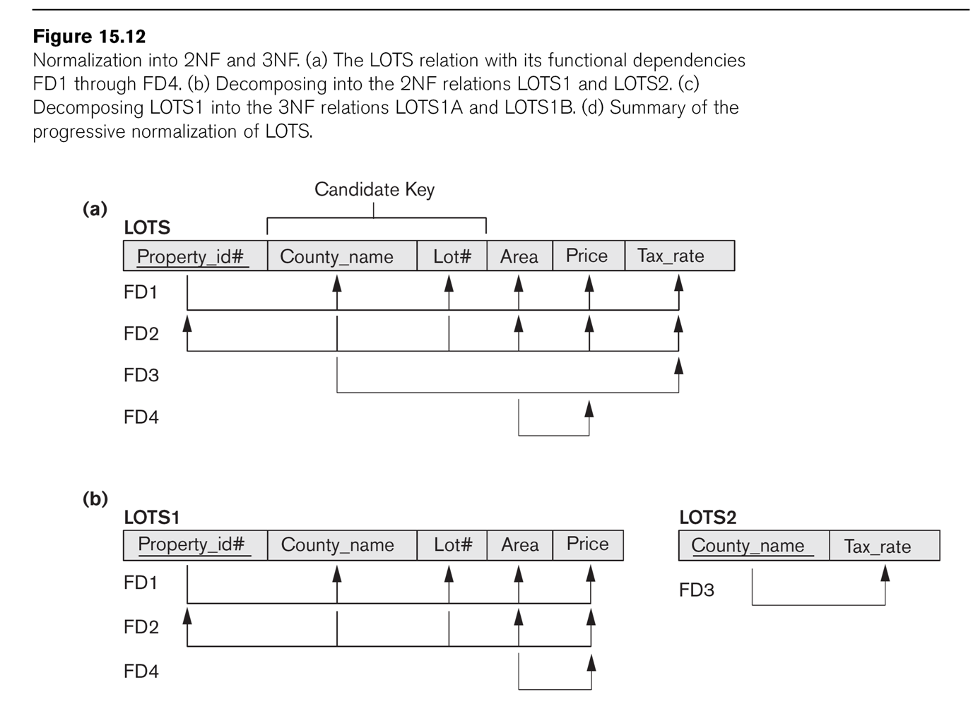
Attributes for LOTS are

property_ID
county
lot_num
area
price
tax_rate

The primary key is property_ID, and ⟨county,lot_num⟩ is also a key. These are functional dependencies FD1 and FD2 respectively. We also have
FD3: county ⟶ tax_rate
FD4: area ⟶ price
(For farmland, FD4 is not completely unreasonable, at least if price refers to the price for tax purposes. In Illinois, the formula is tax_price = area × factor_determined_by_soil_type).

2NF fails because of the dependency county ⟶ tax_rate; FD4 does not violate 2NF. E&N suggest the decomposition into LOTS1(property_ID, county, lot_num, area, price) and LOTS2(county, tax_rate).

We can algorithmically use a 2NF-violating FD to define a decomposition into new tables. If X⟶A is the FD, we remove A from table R, and construct a new table with attributes those of X plus A. E&N did this above for FD3: county ⟶ tax_rate.

Before going further, perhaps two points should be made about decomposing too far. The first is that all the functional dependencies should still appear in the set of decomposed tables; the second is that reassembling the decomposed tables with the "obvious" join should give us back the original table, that is, the join should be lossless.

A lossless join means no information is lost, not that no records are lost; typically, if the join is not lossless then we get back all the original records and then some.

In Fig 15.5 there was a proposed decomposition into EMP_LOCS(ename, plocation) and EMP_PROJ1(ssn,pnumber,hours,pname,plocation). The join was not lossless.

Third Normal Form

Third Normal Form (3NF) means that the relation is in 2NF and also there is no dependency X⟶A for nonprime attribute A and for attribute set X that does not contain a candidate key (ie X is not a superkey). In other words, if X⟶A holds for some nonprime A, then X must be a superkey. (For comparison, 2NF says that if X⟶A for nonprime A, then X cannot be a proper subset of any key, but X can still overlap with a key or be disjoint from a key.)

2NF: If K represents the set of attributes making up the primary key, every nonprime attribute A (that is an attribute not a member of any key) is functionally dependent on K (ie K⟶A), but that this fails for any proper subset of K (no proper subset of K functionally determines A).

3NF: 2NF + there is no dependency X⟶A for nonprime attribute A and for an attribute set X that does not contain a key (ie X is not a superkey).

normal forms diagrams

Recall that a prime attribute is an attribute that belongs to some key. A nonprime attribute is not part of any key. The reason for the nonprime-attribute restriction on 3NF is that if we do have a dependency X⟶A, the general method for improving the situation is to "factor out" A into another table, as below. This is fine if A is a nonprime attribute, but if A is a prime attribute then we just demolished a key for the original table! Thus, dependencies X⟶A involving a nonprime A are easy to fix; those involving a prime A are harder.

If X is a proper subset of a key, then we've ruled out X⟶A for nonprime A in the 2NF step. If X is a superkey, then X⟶A is automatic for all A. The remaining case is where X may contain some (but not all) key attributes, and also some nonkey attributes. An example might be a relation with attributes K1, K2, A, and B, where K1,K2 is the key. If we have a dependency K1,A⟶B, then this violates 3NF. A dependency A⟶B would also violate 3NF.

Either of these can be fixed by factoring out: if X⟶A is a functional dependency, then the result of factoring out by this dependency is to remove column A from the original table, and to create a new table ⟨X,A⟩. For example, if the ⟨K1, K2, A, B⟩ has dependency K1,A⟶B, we create two new tables ⟨K1, K2, A⟩ and ⟨K1, A, B⟩. If we were factoring out A⟶B, we would create new tables ⟨K1, K2, A⟩ and ⟨A,B⟩. Both the resultant tables are projections of the original; in the second case, we also have to remove duplicates.

Note again that if A were a prime attribute, then it would be part of a key, and factoring it out might break that key!

One question that comes up when we factor is whether it satisfies the nonadditive join property (or lossless join property): if we join the two resultant tables on the "factor" column, are we guaranteed that we will recover the original table exactly? The answer is yes, provided the factoring was based on FDs as above. Consider the decomposition of R = ⟨K1, K2, A, B⟩ above on the dependency K1,A⟶B into R1 = ⟨K1, K2, A⟩ and R2 = ⟨K1, A, B⟩, and then we form the join R1⋈R2 on the columns K1,A. If ⟨k1,k2,a,b⟩ is a record in R, then ⟨k1,k2,b⟩ is in R1 and ⟨k1,a,b⟩ is in R2 and so ⟨k1,k2,a,b⟩ is in R1⋈R2; this is the easy direction and does not require any hypotheses about constraints.

The harder question is making sure R1⋈R2 does not contain added records. If ⟨k1,k2,a,b⟩ is in R1⋈R2, we know that it came from ⟨k1,k2,a⟩ in R1 and ⟨k1,a,b⟩ in R2. Each of these partial records came from the decomposition, so there must be b' so ⟨k1,k2,a,b'⟩ is in R, and there must be k2' so ⟨k1,k2',a,b⟩ is in R, but in the most general case we need not have b=b' or k2=k2'. Here we use the key constraint, though: if ⟨k1,k2,a,b⟩ is in R, and ⟨k1,k2,a,b'⟩ is in R, and k1,k2 is the key, then b=b'. Alternatively we could have used the dependency K1,A⟶B: if this dependency holds, then it means that if R contains ⟨k1,k2,a,b⟩ and ⟨k1,k2,a,b'⟩, then b=b'.

This worked for either of two reasons: R1 contained the original key, and R2's new key was the lefthand side of a functional dependency that held in R.

In general, if we factor a relation R=⟨A,B,C⟩ into R1=⟨A,B⟩ and R2=⟨A,C⟩, by projection, then the join R1⋈R2 on column A might be much larger than the original R. As a simple example, consider Works_on = ⟨essn,pno,hours⟩; if we factor into ⟨essn,pno⟩ and ⟨pno,hours⟩ and then rejoin, then essn,pno will no longer even be a key. Using two records of the original data,

123456789	1	32.5
453453453	1	20

we see that the factored tables would contain ⟨123456789,1⟩ and ⟨1,20⟩, and so the join would contain ⟨123456789,1,20⟩ violating the key constraint.

The relationship EMP_DEPT of EN fig 15.11 is not 3NF, because of the dependency dnumber ⟶ dname (or dnumber ⟶ dmgr_ssn).
dependencies

Can we factor this out?

The LOTS1 relation above (EN fig 15.12) is not 3NF, because of Area ⟶ Price. So we factor on Area ⟶ Price, dividing into LOTS1A(property_ID, county,lot_num,area) and LOTS1B(area,price). Another approach would be to drop price entirely, if it is in fact proportional to area, and simply treat it as a computed attribute.

4343

Multiple factoring outcomes

Consider a relation ⟨K1, K2, A, B, C⟩ where K1,K2 is the key and we have dependencies K1⟶B and B⟶C. If we try to put into 2NF first, by "factoring out" K1⟶B, we get tables ⟨K1,K2,A,C⟩ and ⟨K1,B⟩; the dependency B⟶C is no longer expressible in terms of the tables. But if we start by factoring out B⟶C, we get ⟨K1,K2,A,B⟩ and ⟨B,C⟩; we can now factor out K1⟶B which yields relations ⟨K1,K2,A⟩, ⟨K1,B⟩ and ⟨B,C⟩; all functional dependencies have now been transformed into key constraints. Factoring can lose dependencies, or, more accurately, make them no longer expressible except in terms of the re-joined tables.

An aid to dealing with this sort of situation is to notice that in effect we have a three-stage dependency: K1⟶B⟶C. These are often best addressed by starting with the downstream (B⟶C) dependency.

Boyce-Codd Normal Form

BCNF requires that whenever there is a nontrivial functional dependency X⟶A, then X is a superkey, even if A is a prime attribute. It differs from 3NF in that 3NF requires either that X be a superkey or that A be prime (a member of some key). To put it another way, BCNF bans all nontrivial nonsuperkey dependencies X⟶A; 3NF makes an exception if A is prime.

As for 3NF, we can use factoring to put a set of tables into BCNF. However, there is now a serious problem: by factoring out a prime attribute A, we can destroy an existing key constraint! This is undesirable.

The canonical example of a relation in 3NF but not BCNF is ⟨A, B, C⟩ where we also have C⟶B. Factoring as above leads to ⟨A, C⟩ and ⟨C, B⟩. We have lost the key A,B! However, this isn't quite all it appears, because from C⟶B we can conclude A,C⟶B, and thus that A,C is also a key, and might be a better choice of key than A,B.

LOTS1A from above was 3NF and BCNF. But now let us suppose that DeKalb county lots have sizes <= 1.0 acres, while Fulton county lots have sizes >1.0 acres; this means we now have an additional dependency FD5: area⟶county. This violates BCNF, but not 3NF as county is a prime attribute. (The second author Shamkant Navathe is at Georgia Institute of Technology so we can assume DeKalb County is the one in Georgia, and hence is pronounced "deKAB".)

If we fix LOTS1A as in Fig 15.13, dividing into LOTS1AX(property_ID,area,lot_num) and LOTS1AY(area,county), then we lose the functional dependency FD2: (county,lot_num)⟶property_ID.

Where has it gone? This was more than just a random FD; it was a candidate key for LOTS1A.

All databases enforce primary-key constraints. One could use a CHECK statement to enforce the lost FD2 statement, but this is often a lost cause.

CHECK (not exists (select ay.county, ax.lot_num, ax.property_ID, ax2.property_ID
    from LOTS1AX ax, LOTS1AX ax2, LOTS1AY ay
    where ax.area = ay.area and ax2.area = ay.area       // join condition
    and ax.lot_num = ax2.lot_num
    and ax.property_ID <> ax2.property_ID))

We might be better off ignoring FD5 here, and just allowing for the possibility that area does not determine county, or determines it only "by accident".

Generally, it is good practice to normalize to 3NF, but it is often not possible to achieve BCNF. Sometimes, in fact, 3NF is too inefficient, and we re-consolidate for the sake of efficiency two tables factored apart in the 3NF process.

Fourth Normal Form

Suppose we have tables ⟨X,Y⟩ and ⟨X,Z⟩. If we join on X, we get ⟨X,Y,Z⟩. Now choose a particular value of x, say x0, and consider all tuples ⟨x0,y,z⟩. If we just look at the y,z part, we get a cross product Y0×Z0, where Y0={y in Y | ⟨x0,y⟩ is in ⟨X,Y⟩} and Z0={z in Z | ⟨x0,z⟩ is in ⟨X,Z⟩}. As an example, consider tables EMP_DEPENDENTS = ⟨ename,depname⟩ and EMP_PROJECTS = ⟨ename,projname⟩:

EMP_DEPENDENTS

ename	depname
Smith	John
Smith	Anna

EMP_PROJECTS

ename	projname
Smith	projX
Smith	projY

Joining gives

ename	depname	projname
Smith	John	X
Smith	John	Y
Smith	Anna	X
Smith	Anna	Y

Fourth normal form attempts to recognize this in reverse, and undo it. The point is that we have a table ⟨X,Y,Z⟩ (where X, Y, or Z may be a set of attributes), and it turns out to be possible to decompose it into ⟨X,Y⟩ and ⟨X,Z⟩ so the join is lossless. Furthermore, neither Y nor Z depend on X, as was the case with our 3NF/BCNF decompositions.

Specifically, for the "cross product phenomenon" above to occur, we need to know that if t1 = ⟨x,y1,z1⟩ and t2 = ⟨x,y2,z2⟩ are in ⟨X,Y,Z⟩, then so are t3 = ⟨x,y1,z2⟩ and t4 = ⟨x,y2,z1⟩. (Note that this is the same condition as in E&N, 15.6.1, p 533, but stated differently.)

If this is the case, then X is said to multidetermine Y (and Z). More to the point, it means that if we decompose into ⟨X,Y⟩ and ⟨X,Z⟩ then the join will be lossless.

Are you really supposed even to look for things like this? Probably not.

Fifth Normal Form

5NF is basically about noticing any other kind of lossless-join decomposition, and decomposing. But noticing such examples is not easy.

16.4 and the problems of NULLs

"There is no fully satisfactory relational design theory as yet that includes NULL values"

[When joining], "particular care must be devoted to watching for potential NULL values in foreign keys"

Unless you have a clear reason for doing otherwise, don't let foreign-key columns be NULL. Of course, we did just that in the EMPLOYEE table: we let dno be null to allow for employees not yet assigned to a department. An alternative would be to create a fictional department "unassigned", with department number 0. However, we then have to assign Department 0 a manager, and it has to be a real manager in the EMPLOYEE table.