Modulation and Transmission
Peter Dordal, Loyola University CS Department
How do we transmit sound (or any other analog or digital signal) using
electromagnetic waves? We modulate the EM wave (the
carrier) in order to encode the signal. The result no longer is a single
frequency; it is a band of frequencies. This spreading of
the single-frequency carrier to a band of frequencies is fundamental.
If we are sending the signal a long way (over transmission
lines), then we may very well also need to modulate some form of carrier. In
the digital context, this is sometimes known as encoding.
Example
Suppose we want to transmit a square wave, alternating from -1 to +1. We
have a band-width of 4 Mhz. How does the data rate ("bandwidth" in the
digital sense) compare to the band-width in the spectrum sense? The simple
modulation here is an attempt to generate a square wave out of sine waves.
Case 1: we use sin(2𝜋ft) + (1/3)sin(2𝜋(3f)t) + (1/5)sin(2𝜋(5f)t) (that
is, three terms of the Fourier series), where f = 1 Mhz.
Look at this with fourier.xls: does it look squarish?
The frequencies are 1 Mhz, 3 Mhz and 5 Mhz. The band-width is 5-1 = 4 Mhz.
The data rate is 2 Mbps (sort of; we are sending 1 M 1-bits and 1 M 0-bits
per second)
Note dependence on notion of what waveform is "good enough"
Case 2: If we double all the frequencies to 2 MHz, 6 MHz, 10 MHz, we get
band-width 8MHz, data rate 4Mbps. This is the same as above with f=2 Mhz.
Case 3: We decide in the second case that we do not
need the 10 MHz component, due to a more accurate receiver. The base
frequency is f = 2MHz, frequencies 2MHz, 6MHz, band-width is now 6MHz - 2MHz
= 4MHz, data rate: 4Mbps
Look at this with fourier.xls.
Note that we're really not carrying data in a meaningful sense; we can't
send an arbitrary sequence of 0's and 1's this way. However, that's done
mostly to simplify things.
Note also the implicit dependence on bandwidth of the fact that we're
decomposing into sinusoidal waves.
Voice transmission: frequency band-width
~ 3-4kHz (eg 300 Hz to 3300 Hz)
64Kbps encoding (8 bits sampled 8000 times a second)
Modems have the reverse job: given the band-width of ~3 kHz, they have to
send at 56 kbps!
Note: we're looking at DISCRETE frequency spectrum (periodic signals).
CONTINUOUS frequency spectrum also makes mathematical sense, but is kind of
technical
Note that frequency-domain notion depends on fundamental theorem of Fourier
analysis that every periodic function can be expressed as sum of sines &
cosines (all with period an integral multiple of original)
Band-width of voice: <=4 kHz
This is quite a different meaning of band-width from the digital usage,
where a 64kbps channel needs a bandwidth of 64kbps.
But if we wanted to encode the digitized voice back into an analog voice
band-width, we'd have to encode 16 bits per cycle (Hertz), which is a little
tricky.
Amplitude modulation & band-width
Note that AM modulation (ALL
modulation, in fact) requires a "band-width"; ie range of frequencies. This
will be very important for cellular.
AM:amplitude = [1+data(t)]*sin(2𝜋ft)
f is "carrier" high frequency; eg 100,000
If data(t) = sin(2𝜋gt), g a much lower frequency (eg 1000)
Then sin(2𝜋ft)*sin(2𝜋gt) = 0.5 cos(2𝜋(f-g)t) - 0.5 cos(2𝜋(f+g)t)
band of frequencies: (f-g) to (f+g)
band-width: 2g
Example: beats+modulation.xls,
beats+modulation.ods
The sincfilter.ods
spreadsheet, demonstrating filtering.
Note that most of the low-pass filtering is done within the first full
cycle.
Discussion of the graph
Transmission
analog transmission: needs
amplifiers to overcome attenuation
digital transmission:
store-and-forward switches?
Switches do signal regeneration, not amplification; noise is NOT added. BUT:
we need them a lot more often.
data may need some form of encoding:
analog may use something like AM modulation, or equalization.
Digital encoding: NRZ is basic (1=on, 0=off), but isn't good in real life.
Analog data:
Analog signal: commonly some form
of modulation on a different frequency
Digital signal: something like PCM
sampling
Digital data:
Analog signal: this is what modems
generate
Digital signal: we need some form
of encoding.
Data: the original data format
Signal: the signal actually
transmitted
Transmission: how we handle that signal on the wire.
analog v data v (encoding | transmission)
Note analog data / analog signal is an odd case.
See http://intronetworks.cs.luc.edu/current/html/links.html#encoding-and-framing
as a reference on encoding of (short-haul) digital signals on a wire.
Signals v Transmission:
Normally these should match. Note special case of analog signal / digital
transmission, which is taken to mean that the analog signal encodes a
digital signal in a way that the repeater can decode and re-encode.
Transmission impairments
- Attenuation
- high-frequency attenuation: signal distortion
- Delay distortion
- Noise
- crosstalk (noise from other signals)
- impulse noise (eg noise from electrical appliances)
Attenuation
1. need strength for reception
Ethernet problem with detecting collisions
2. need strength above noise level
3. attenuation increases with frequency, leading to distortion
"loading coils" in voice telephony: cut off frequencies outside of a desired
range; tremendous out-of-band attenuation
attenuation measured in dB; dB per unit distance
Here is a graph from Stallings showing the relative attenuation of voice
frequencies:
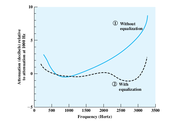
Note use of equalization to make up for high-frequency loss
Brief review of decibels: logarithmic scale of relative
power:
db = 10 log10 (P/Pbaseline)
3 dB = 2× log10(2) = .30103
5 dB = 3×
7 dB = 5× (5× = 10×/2×; 7 = 10-3)
10 dB = 10×
20 dB = 100×
Attenuation problems 1 & 2 above can be addressed with amplification.
3rd problem introduces fundamental distortion; digitization solves this but
analog equalization can work too.
Digital: high-frequency attenuation => signal degradation
Attenuation: leads to distortion of relative frequency strengths
Delay Distortion (like differential
frequency attenuation, but different): different (sine) frequencies travel
at different speeds.
Again, this leads to digital signal degradation, and some audio distortion.
Noise
Thermal noise:
N (watts) = kTB, B=band-width, T=temp, k=Boltzmann's constant (small!).
Thermal noise is relevant for satellite transmission, but other sources of
noise are usually more important for terrestrial transmission.
Note that thermal noise is proportional to the analog bandwidth; ie, it
affects all frequencies identically.
It is often more convenient to use logarithms (base 10):
Noise in dBW = log(k) + log(T) + log(B)
log(k) = -228.6 dBW
Suppose the temperature is 300K (27 degrees C) and the band-width is 20 MHz.
Then the thermal noise is
-228.6 + 10 log 300 + 10 log 20,000,000 = -228.6 + 24.8 +
73 = -133.5 dBW
dBW is the difference (in decibels) from a 1 Watt reference signal.
Intermodulation noise
This is the noise created by two signals interacting, in the same medium
Brief discussion on why it isn't universal.
Intermodulation noise requires some nonlinear
interaction between the signals!
A linear combination of frequencies f1 and f2 (ie just transmitting them
side-by-side in space) does not
produce energy at f1+f2.
Crosstalk
Noise created by two signals interacting, on adjacent wires
Impulse noise
- Fridge story
- Bad for data
- Most significant noise for ordinary wiring
Interference (a form of impulse noise, from sharers of your frequency range)
Somebody else is using your frequency. Perhaps to make microwave
popcorn. (Or perhaps you are simply driving around in the country
listening to the radio.)
Other sources of noise:
- poor connectors
- cosmic rays / sunspots (form of impulse noise)
- signal reflections from connectors/taps
Channel capacity
Nyquist's Theorem: the signal
rate is the rate of sending data symbols.
Nyquist's theorem states that
maximum binary signal
rate = 2 B
Where B is the width of the frequency band (that is, the "band-width").
This can be hard to realize in practice.
Signal rate v data rate: if we use binary signaling (binary encoding), then
this means
max data rate = 2 B
(binary version)
We might also send symbols (signal elements) each encoding L bits,
in which case the data rate is L×signal_rate. One way to do this is to use multi-level
encoding, using M=2L distinct signal values (eg
distinct amplitudes, etc). In this case we have
max data rate = 2 B × log2(M)
(multi-level version)
For binary signals, M=2 and log2(M)=1, so we just get the
binary-version formula. Log2(M) is the number of bits needed to
encode M, that is, the number of bits per symbol.
Signal rate is sometimes called "modulation rate". It is traditionally
measured in baud. Note that for a
56k "baud" modem, it's the data rate
that is 56kbps; the signaling rate is 8000/sec.
Compare Nyquist to the Sampling Theorem, which says that if a sine wave has
frequency B, then it can be exactly reproduced if it is sampled at a rate of
2B. (Note: the sampling theorem allows for exact reproduction only if the
sampled values are exact. In real life, the sampled values are digitized,
and thus "rounded off"; this is called quantizing
error.)
Basis of Nyquist's theorem: fundamental mathematics applied to individual
sine waves.
The data rate is sometimes called "bandwidth" in non-analog settings.
The Nyquist limit does not take noise
into account.
Note that if we are talking about a single sin(x), then analog band-width =
0! sin(x) does not carry any
useful information.
Example 1: M=8, log2(M) = 3. Max data rate is 6B.
With M levels, we can carry log2(M) bits where we used to only
carry 1 bit.
Why can't we just increase the bits per signal indefinitely, using
multi-level encoding with more and more levels?
Answer: noise.
The Shannon-Hartley Theorem uses
the noise level to give an upper bound on the communications throughput.
If S is the signal power and N is the noise power, then the signal-to-noise
ratio, SNR, is S/N. This is often measured in dB, though in the formula
below we want the actual ratio (25 dB = 300×)
Shannon-Hartley claim:
C ≤ B log2(SNR + 1)
where B = band-width, C = maximum channel capacity
Example: 3000Hz voice bandwidth, S/N = 30 dB, or a ratio of 1000.
C = 3000*log2(1000) = 3000*10 = 30kbps
Note that increasing signal strength does tend to increase noise as well.
Also, increasing band-width increases noise more or less in proportion. So:
increasing B does lead to more thermal noise, and thus by Nyquist's formula
SNR will decrease.
Here's a quick attempt to justify the Shannon-Hartley formula, borrowed from
www.dsplog.com/2008/06/15/shannon-gaussian-channel-capacity-equation.
It essentially derives Hartley's original formula. Let us start with the
assumption that Sv is the maximum signal voltage, and Nv
is the range of noise voltage; noise itself ranges from −Nv/2 to
+Nv/2. Nv is much smaller than Sv. We'd
like to choose an M so the M different voltages 0, Sv/(M-1), 2Sv/M,
..., (M-1)Sv/(M-1) are all distinct. This means that the step
between two adjacent voltages is at least as large as Nv, as the
upper voltage can have Nv/2 subtracted while the lower voltage
can have Nv/2 added. This means Sv/(M-1) = Nv,
or
M = Sv/Nv+1 = (Sv+Nv)/Nv
The number of bits we can send with M levels is log2(M) = log2(Sv/Nv+1).
We're using voltages here; we really want to use power, which, all else
being equal, is proportional to the square of the voltage. Let S = Sv2
and N = Nv2, so (S/N)1/2 = Sv/Nv.
We now have, ignoring the "+1" because S/N is large,
log2M = (1/2) log2(S/N)
If B is the bandwidth then Nyquist's theorem says in effect that the maximum
symbol rate is 2B. This means that our data rate is 2B × (1/2) log2(S/N)
= B log2(S/N).
We've said nothing about the idea that noise is statistically distributed
following the Gaussian distribution. But this is a first step.
Let us equate the Shannon and Nyquist formulas for C:
C = 2B log2(M) ≤ B log2(SNR+1)
M2 ≤ SNR+1
Suppose we take SNR = 251×; from the above we can infer that we can have at
most M=16 signal levels.
56kbps modem: C=56kbps, B=3100Hz. C/B = 18
18 = log2(1 + SNR); SNR ~ 218 = 260,000 = 54 dB
Nyquist and 56Kbps modem: B=4kHz; 128 = 27 levels
Shannon and 28/56Kbps modems
Eb/N0
noise is proportional to bandwidth; let N0 = noise power per
Hertz.
Eb = energy per bit of signal (eg wattage of signal ×
time-length of bit; this decreases with increased signaling rate (shorter
time)) or lower average signal energy.
Ratio is Eb/N0
Note that this is a dimensionless quantity, though as a ratio of energy
levels it is often expressed (logarithmically) in dB.
bit error rate decreases as this increases; significant for optical fiber
designers
We will often assume N0 is all thermal noise, equated to kB, but the notion makes sense when there
is other noise too.
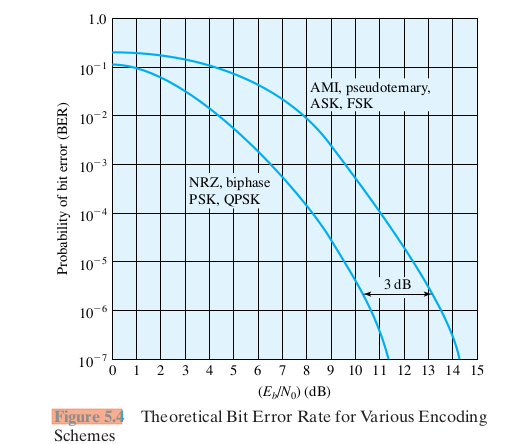
Here is figure 5.4 from Stallings involving BER v Eb/N0:
Transmission Media
EM spectrum:
10
100
1000 voice
104
105
106
AM radio
107
shortwave
108
FM radio, television
109
Wi-Fi, microwave ovens
1010
microwaves
1011
1012
Low end of infrared
1013
1014
Red end of visible light
Attenuation of various media (from Stallings)
Twisted pair (loading coils) 0.2 dB/km at 1kHz
Twisted pair (voice-grade) 0.7 dB/km at 1kHz, 25 dB/km at
1 MHz
Cat-3
12 dB/km at 1 MHz
Coax
2dB/km at 1 MHz
Coax (fat)
7 dB/km at 10 MHz
Fiber
0.2 - 0.5 dB/km
consider attenuation & interference for the following.
Note: attenuation measured in dB/km! What are the implications of this!
At 16 mHz, attenuation per tenth of
a km:
13 dB (cat 3)
8 dB (cat 5) (80 dB/km)
Why is it TWISTED??
summary: Coax has less attenuation, much less crosstalk/interference, but is
$$
fiber
fiber modes
- step-index multimode: reflection off fiber surface
- graded-index multimode: light is refracted away from surface due to
changes in refractive index
- single-mode: single light ray down the center of the fiber
light source: lasers or LEDs (the latter is cheaper)
ADSL issues:
Stallings table 4.2: Cat-3 twisted pair has an attenuation of 2.6dB/100m!!
(at 1 mHz)
Over the maximum run of 5 km, this works out to an incredible 90dB loss! And
residential phone lines are not twisted-pair.
384Kbps: 17,000 feet
1.5mbps: 12,000 feet
ADSL must deal with tremendous
signal attenuation!
Thermal noise becomes very serious!
Antennas
Satellite note: I used to have satellite internet.
My transmitter was 2 watts. This reached 23,000 miles.
The central problem with satellite phone (and internet) links is delay. The
round-trip distance (up-down-up-down) is 4x23,000 miles, for a minimum
propagation delay of 495 ms. For Internet, there was usually an additional
500 ms of queuing delay.
Frequencies: < 1.0 gHz: noisy
> 10 gHz: atmospheric attenuation
Wi-fi uses the so-called "ISM" band, at around 2.4 gHz
4.3: propagation
High-frequency is line-of-sight, but low frequency (<= ~ 1 mHz) bends
In between is "sky-wave" or ionospheric skip (2-30mHz)
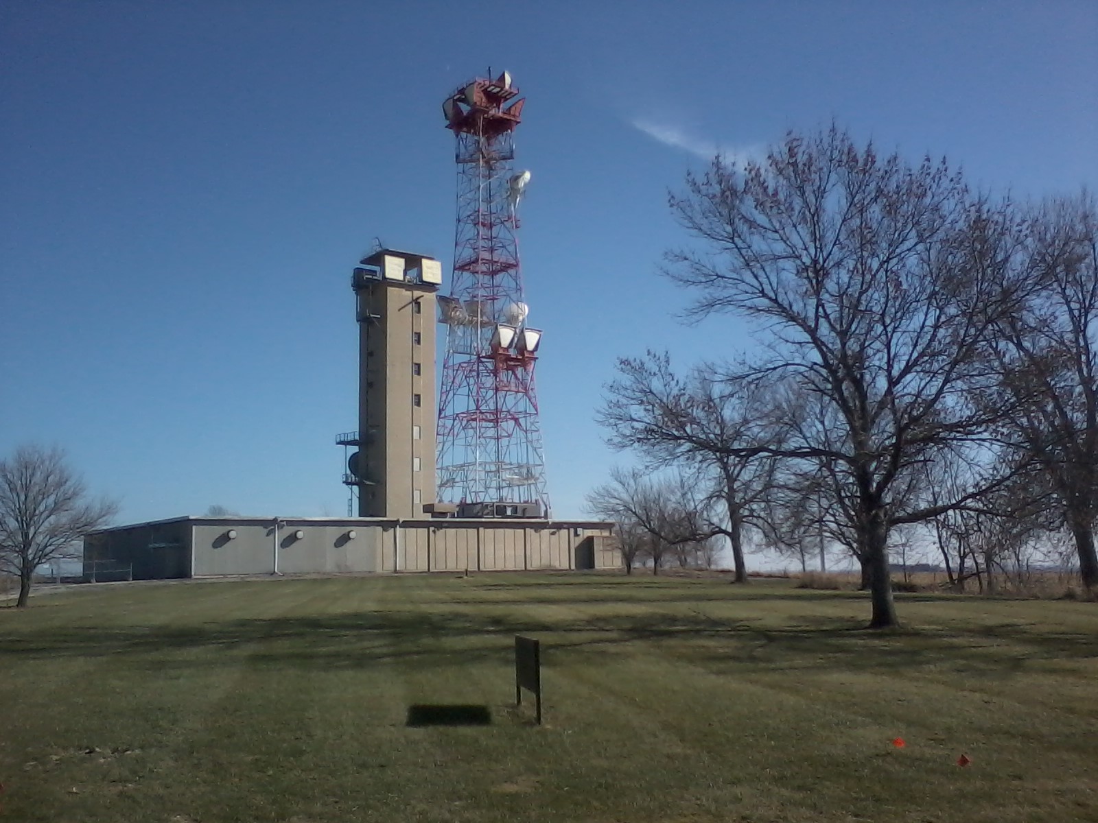
Once upon a time, AT&T had chains of microwave towers, 40-50 miles
apart. They would relay phone calls. They're obsolete now, replaced by
fiber. The concrete tower in the picture below, built in 1950, is the
original phone microwave-relay tower; the newer steel tower arrived in 1957.
(Further information about this particular site can be found at long-lines.net/places-routes/LeeIL;
information about the entire system can be found at long-lines.net.)
The single-story base building is huge;
it was built to house vacuum-tube electronics and early transistor
technology. Nowadays the electronics fit within the base of each antenna.
Suppose you could have 100 mHz of band width (eg 2.5-2.6 gHz). At 4 kHz per
call, that works out to 25,000 calls. That many calls, at 64kbps each,
requires a 1.6-gbit fiber line. In the SONET hierarchy, that just below
OC-36/STS-36/STM-12. Single fiber lines of up to STM-1024 (160 Gbps; almost
100 times the bandwidth) are standard, and are usually installed in
multiples.
Is it cheaper to bury 50 miles of cable, or build one tower?
Now suppose you decide (before construction begins) that you need 10× more
capacity. What then?
Line-of-sight:
Attenuation, inverse-square v exponential
water vapor: peak attenuation at 22gHz (a 2.4gHz microwave is not
"tuned" to water)
rain: scattering
oxygen: peak absorption at 60 gHz
cell phones: 824-849mhz
pcs: 1.9ghz
Attenuation along a wire (coax, twisted pair, or anything
else) is exponential, while wireless
attenuation is proportional to the square of the distance, meaning that in
the long run wire attenuation becomes much more significant than wireless.
Every time you double the distance with wireless, the signal strength goes
down by a factor of 4, which is a 6 dB loss. Suppose a cable has a loss of 3
dB per 100 m (factor of 2). Suppose the wired signal is 10 db ahead at 100
m. We get the following
| distance |
wired |
wireless |
| 100 m |
0 db |
-10 db |
| 200 m |
-3 db |
-16 db |
| 400 m |
-9 db |
-22 db |
| 800 m |
-21 db |
-28 db |
| 1600 m |
-45 db |
-34 db |
Starlight (a form of wireless) is detectable at distances of 100's of
light-years.
Techniques for Modulation and Encoding
5.1 digital data/digital signal
NRZ is the "simple" encoding. But on
short-haul links it has problems with clock drift. It has additional
problems with long-haul encodings.
See also http://intronetworks.cs.luc.edu/current/html/links.html#encoding-and-framing about the encoding of short-haul
digital signals on a wire.
data rate v modulation rate: these are often not the same
(ethernet: data rate 10Mbps, modulation rate 20Mbaud)
phone modems: data rate 56kbps, modulation rate 7kbaud
RZ, NRZ
issues:
clocking
analog band width: avoid needing
waveforms that are too square
DC component (long distances don't
like this)
noise
NRZ flavors
inversion (NRZ-I) v levels (NRZ-L)
differential coding (inversion) may be easier to detect than comparison to
reference level
Also, NRZ-I guarantees that long runs of 1's are self-clocked
Problems:
DC component: non-issue with short (LAN) lines, larger issue with long lines
losing count / clocking (note that NRZ-I avoids this for 1's)
Requirements:
- no DC component
- no long runs of 0 (or any constant voltage level)
- no reduction in data rate through insertion of extra bits
bipolar (bipolar-AMI): 1's are alternating +/-; 0's are 0
Fixes DC problem! Still 0-clocking problem
Note that bipolar involves three levels: 0, -1, and +1.
biphase: (bi = signal + clock)
Example: Manchester (10mbps ethernet)
10mbps bit rate
20mbps baud rate (modulation rate)
bipolar-8-zeros (B8ZS)
This is what is used on most North American T1 lines (I'm not sure about T3,
but probably there too)
1-bits are still alternating +/-; 0-bits are 0 mostly.
If a bytes is 0, that is, all the bits are 0s (0000 0000), we replace it
with 000A B0BA, where A = sign of previous pulse and B=-A.
This sequence has two code
violations. The receiver detects these code violations & replaces the
byte with 0x00.
Note the lack of a DC component
Example: decoding a signal
Bipolar-HDB3: 4-bit version of B8ZS
4b/5b
4-bit
data
|
5-bit
code
|
0000
|
11110 |
0001
|
01001 |
0010
|
10100 |
0011
|
10101 |
...
|
|
1100
|
11010 |
1101
|
11011 |
1110
|
11100 |
1111
|
11101 |
IDLE
|
11111 |
DEAD
|
00000 |
HALT
|
00100 |
4b/5b involves binary levels,
unlike bipolar. It does entail a 20% reduction in the data rate.
It is used in 100-mbit Ethernet
Fig 5.3 (8th, 9th edition): spectral density of encodings. Spectral density
refers to the band-width that the signal needs.
Lowest to highest:
- biphase (Manchester, etc)
- AMI,
- B8ZS
Latter is narrower because it guarantees more transitions
=> more consistent frequency
Fig 5.4: theoretical bit error rate
biphase is 3 dB better than AMI: not sure why. This means that, for the same
bit error rate, biphase can use half the power per bit.
HDLC Bit Stuffing
The HDLC protocol sends frames back-to-back on a serial line; frames are
separated by the special bit-pattern 01111110 = 0x7E. This is, however, an
ordinary byte; we need to make sure that it does not appear as data. To do
that, the bit stuffing technique is
used: as the sender sends bits, it inserts an extra 0-bit after every 5 data
bits. Thus the pattern 01111110 in data would be sent as 011111010.
Here is a longer example:
data:
0111101111101111110
sent as: 011110111110011111010
The receiver then monitors for a run of 5 1-bits; if the next bit is 0 then
it is removed (it is a stuffed bit); if it is a 1 then it must be part of
the start/stop symbol 01111110.
Some consequences:
- We have guaranteed a maximum run of 6 1-bits; if we interchange 0's
and 1's and use NRZ-I, bit-stuffing has solved the clocking problem for
us.
- The transmitted size of an HDLC data unit depends on the particular
data, because the presence of stuffed bits depends on the particular
data. This will ruin any exact synchronization we had counted on; for
example, we cannot use HDLC bit-stuffing to encode voice bytes in a DS0
line because the extra stuffed bits will throw off the 64000-bps rate.
- The data sent, and the 01111110 start/stop symbol, may no longer align
on any byte boundaries in the underlying transmission bitstream.
see also http://intronetworks.cs.luc.edu/current/html/links.html#framing.
Analog data / Digital signal
(Stallings 5.3)
sampling theorem: need to sample at twice the max frequency, but not more
basic idea of PCM: we sample at regular intervals (eg 1/8000 sec), digitize
the sample amplitude, and send that.
PCM stands for Pulse Code Modulation; it replaced an earlier analog strategy
called PAM: Pulse Amplitude Modulation. In PAM, the signal was sampled and
then a brief carrier pulse of that amplitude was sent. This is a little like
AM, except the pulses could be short, and time-division-multiplexed (below)
with other voice channels. The C in PCM means that the analog signal was
replaced by a "code" representing its amplitude. This is all meant to
explain why digital sampling, which is what PCM is, gets the word
"modulation" in its name, which is really not applicable.
In the early days, one sampler (PCM encoder) could sample multiple analog
input lines, saving money on electronics.
sampling error v quantization error
nonlinear encoding versus "companding" (compression/expansion)
The voice-grade encoding used in the US is known as 𝜇-law
(mu-law) encoding; 𝜇 is a constant used in the scaling formula, set equal
to 255. We define F(x) as follows, for -1<=x<=1 (sgn(x) = +1 for
x>0 and -1 for x<0):
F(x) = sgn(x)*log(1+𝜇*|x|) / log(1+𝜇),
Note that for -1<=x<=1 we also have -1<=F(x)<=1. If x is the
signal level, on a -1≤x≤1 scale, then F(x) is what we actually transmit.
More precisely, we transmit 128*F(x), rounded off to the nearest 8-bit
integer. The use of F(x) has the effect of nonlinear scaling,
meaning that for x close to 0 there are still a wide range of levels.
Consider the following few values:
F(1)=1, F(-1)=-1, F(0)=0
F(0.5)= .876, × 128 = 112
F(0.1)= .591 × 128 =
76
F(0.01)= .228 × 128 = 29
F(0.001)= .041 × 128 = 5
These last values mean that faint signals (eg, x = 0.001) still get
transmitted with reasonably limited quantizing roundoff. A signal around x =
0.01 can get rounded off by at most 1/2×29 ≃ 0.016; a signal around x =
0.001 gets rounded off by at most 1/2×5 = 0.1. With linear
scaling, a signal level of 0.01 (relative to the maximum) would encode as 1
(0.01 × 128 = 1.28 ≃ 1), and anything fainter would round off to 0.
This is often called companding, for
compression/expanding; note that it is done at the per-sample level. If
everyone's voice energy ranged, say, from 100% down to a floor of 20% of the
maximum, companding wouldn't add anything. But voice energy in fact has a
much wider dynamic range.
Music, of course, has an even larger dynamic range, but musical encoding
almost always uses 16 bits for sampling, meaning that plain linear encoding
can accurately capture a range from 100% down to at least 0.1%. 8-bit 𝜇-law
companding is often considered to be about as accurate, from the ear's
perspective, as 12 or 13-bit linear encoding.
Demo of what happens if you play a 𝜇-law-encoded file without the necessary
expansion: faint signals (including hiss and static) get greatly amplified.
To get sox to accept this, rename cantdo.ulaw to cantdo.raw and then:
play -r 8000 -b 8 -c 1 -e signed-integer cantdo.raw
A-law encoding: slightly different formula, used in Europe.
By comparison to companding, compression may involve
taking advantage of similarities in a sequence of samples. MP3 is
a form of true compression, though it is not used in telephony (because it
is hard to do in real time). G.729 is a high-performance form of true
compression frequently used in voice.
delta modulation: This involves encoding the data as a
sequence of bits, +1 or -1. The signal level moves up by 1 or down by 1,
respectively. This limits how closely the encoded signal can track the
actual signal. I have no idea if this is actually used. It has a bias
against higher frequencies, which is ok for voice but not data
advantage: one bit! However, higher sampling rates are often necessary.
Performance of digital voice encoding:
voice starts out as a 4kHz band-width.
7-bit sampling at 8kHz gets 56kbps, needs 28kHz analog band-width (by
Nyquist)
(Well, that assumes binary encoding....)
BUT: we get
- digital repeaters instead of analog amplifiers
- digital reliability
- no cumulative noise
- can use TDM instead of FDM
- digital switching
voice: often analog=>digital, then encoded as analog signal on the
transmission lines!
Analog data / Analog signal
(Stallings 5.4)
Why modulate at all? The primary reasons are
- to be able to support multiple non-interfering channels (FDM, or
Frequency-Division Multiplexing)
- to be able to take advantage of higher-frequency transmission
characteristics (you can't broadcast voice frequencies!)
AM and FM radio is the classic example. Cellular telephony would be
analog data / digital signal
The simplest is AM.
AM band-width usage is worth noting
new frequencies at carrier +/- signal are generated because of nonlinear
interaction (the modulation process itself).
Single Side Band (SSB): slightly
more complex to generate and receive, but:
- half the band-width
- no energy at the carrier frequency (this is "wasted" energy)
Sound files: beats.wav v modulate.wav
Latter has nonlinearities
(1+sin(sx)) sin(fx) = sin(fx) + sin(sx)sin(fx)
= sin(fx) + 0.5 cos((f-s))x) - 0.5
cos((f+s)x)
reconsider "intermodulation noise". This is nonlinear interactions between
signals, which is exactly what modulation here is all about.
Angle Modulation (FM and PM)
FM is Frequency Modulation; PM is Phase
Modulation. These can be hard to tell apart, visually.
Let m(t) = modulation signal (eg voice or mustic).
The (transmitted) signal is then
A cos (2𝜋ft + 𝜑(t))
FM: k*m(t) = 𝜑'(t) (that is, 𝜑(t) = ∫m(t)dt). If m(t) = c
is constant for an interval, then 𝜑(t) = kct = k1t; that is, we
have the transmitted signal as
A cos (2𝜋ft + kct) = A cos (2𝜋(f+kc/2𝜋) t),
a signal with the fixed (higher) frequency f+kc/2𝜋.
(We are assuming m(t) is a constant level, not a constant frequency)
PM: k*m(t) = 𝜑(t). m(t) = const => 𝜑(t) = const.
We shift phase for the duration of the constant interval, but the base
frequency changes only when m(t) is changing.
See modulation.xls.
Somewhat surprisingly, FM and PM often sound very similar. One reason for
this is that the derivative (and so the antiderivative) of a sine wave is
also a sine wave. There's distortion in terms of frequency, but most voice
frequencies are in a narrow range.
Picture: consider a signal m(t) = 0 0 1 1 1 1 1 1 0 0 0 0
FM,PM both need more band-width than AM
AM: band-width = 2B, B=band-width of orig signal
FM,PM: band-width = 2(β+1)B, where again B = band-width of original signal.
This is Carson's Rule.
For PM, β = npAmax, A_max = max value of m(t) and np
is the "phase modulation index", a quantity proportional to k in the PM rule
k*m(t) = 𝜑(t).
For FM, β = 𝚫F/B, 𝚫F = peak frequency difference. A value of β=2,
for example, would mean that in encoding an audio signal with band-width 4
KHz, the modulated signal varied in frequency by a total range of 8 KHz.
Having β low reduces the band-width requirement, but also increases noise.
Also note that in our β=2, the total band-width needed for the modulated
signal wold be 24 KHz.
Digital data / Analog signal
Stallings 5.2
modems, long lines & fiber
(even long copper lines tend to work better with analog signals)
ASK: AM modulation using something like the NRZ signal as the input. It is a
"naive" encoding, though used for fiber
FSK: FM modulation. 1-bits are transmitted by brief pulses at frequency f1
(that is, A cos(2𝜋f1t)), while 0-bits are transmitted by brief
pulses at another frequency f2. The bit-time must be long enough
that the two frequencies f1 and f2 are easily
distinguished!
On optical fiber, FSK is represented by color shift.
PSK: easier to implement (electrically) than FSK. 0-bits might be sent as A
cos(2𝜋ft), while for 1-bits the waveform might change to A cos(2𝜋ft + 𝜃)
Superficially, ASK appears to have zero analog band-width, but this is not
really the case!
ASK: 1 bit /hertz => 4000 bps max over voice line
1 bit/ 2Hz, 2400 Hz carrier => 1200 bps.
FSK analog band-width = high_freq - low_freq
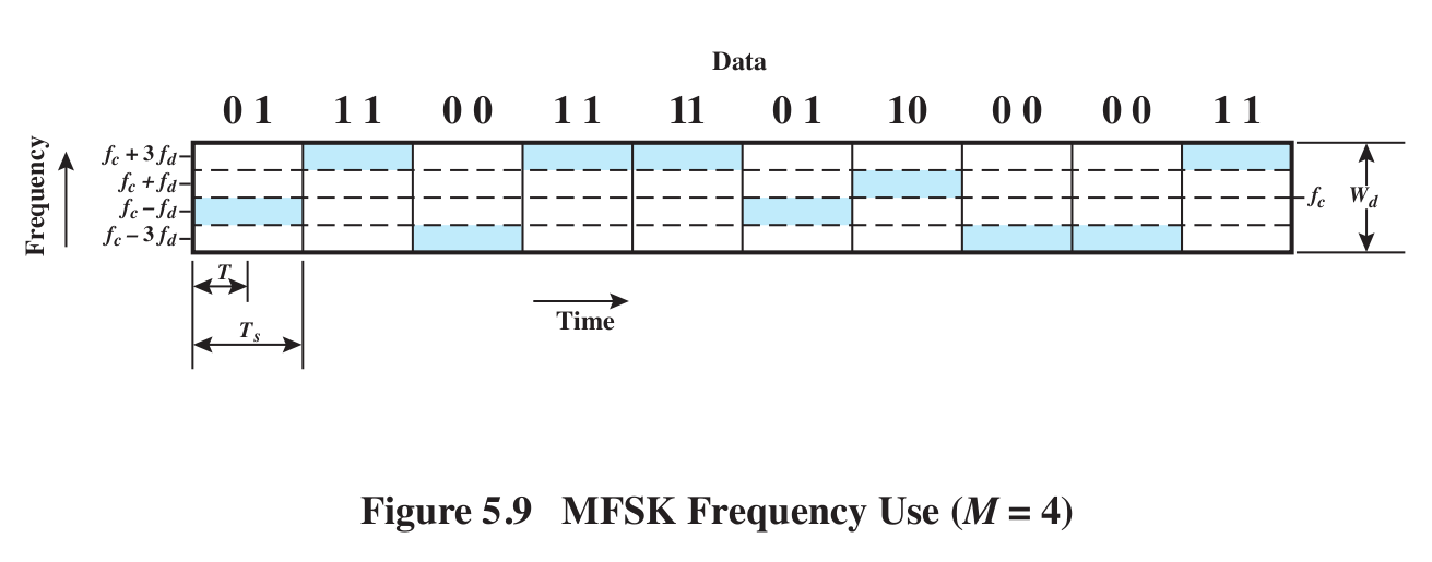
MFSK: we use multiple frequencies to send several bits at
once. If we have four frequencies to use (eg f-3d, f-d, f+d and f+3d, where
f is the "carrier"), then one frequency encodes two bits. We might even
label the frequencies with the bits encoded: f00, f01,
f10, f11.
BFSK v MFSK: fig 5.9 for MFSK.
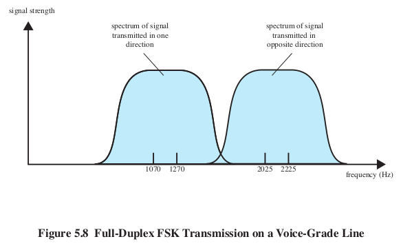
BFSK: fig 5.8: old modems, full-duplex
One direction of the signal might use the frequency band 600-1600 Hz, and
the other direction might use the band 1800-2800 Hz.
MFSK: the trouble is, it takes time
to recognize a frequency (several cycles at least!)
FSK is supposedly more "noise-resistant" than ASK, but fig 5.4 shows the
same graph of Eb/N0 v BER for the two. (PSK is shown 3 dB lower
(better) in the graph)
BPSK: decoding starts to get very nonintuitive!
DPSK: differential, like differential NRZ
QPSK: 4 phase choices, encoding 00, 01, 10, 11
9600bps modem: really 2400 baud; 4 bits per signal element (12 phase angles,
four of which have two amplitude values, total 16 distinct values per
signal, or 4 bits)
Nyquist limit applies to modulation rate: noise reduces it.
56Kbps modems: use PCM directly.
Station gets data 7 bits at a time, every 1/8 ms, and sets the output level
to one of 128 values.
If there is too much noise for the receiver to distinguish all those values,
then use just every other value: 64 values, conveying 6 bits, for 48kbps. Or
32 values (using every fourth level), for 5*8 = 40 kbps.
Quadrature Amplitude Modulation, QAM
This involves two separate signals, sent 90° out of phase and each
amplitude-modulated (ASK) separately. Because the two carriers are 90° out
of phase (eg sin(ft) and cos(ft)), the combined signal can be accurately
decoded.
We will ignore the QAM details.
An Example
The following example is due to Oona Räisänen, via her blog at windytan.com/2014/02/mystery-signal-from-helicopter.html.
We make use of audacity
and the SoX program.
We start with a police helicopter video at youtube.com/watch?v=TCKRe4jJ0Qk.
What is that buzzing noise? The engine? Step 0 is to save the sound track as
an mp3 file (police_chase.mp3), using, say, vidtomp3.com.
Next, using Audacity, convert the mp3 file to .wav format. While we're here,
note the distinctive appearance of the left channel.
The next step is to extract the left channel using
sox police_chase.wav -c 1 left.wav remix 1
Zoom in on the left.wav file. It appears to be a mixture of higher-frequency
and lower-frequency sine waves. The high-frequency wavelength is about .45
ms, making the frequency ~2200 Hz; the lower-frequency wavelength is about
.85 ms, making the frequency ~1200 Hz. These numbers turn out to match the Bell
202 modulation scheme, which uses FSK: data is sent at a rate of
1200 bps, with 1-bits encoded as a single wavelength at 1200 Hz and 0-bits
encoded as 1.83 wavelengths (1/1200 sec) at 2200 Hz. Bell 202 modulation is
still used to transmit CallerID data to analog landline phones.
How do we demodulate the signal? One approach is to apply lowpass and
highpass filters about the midpoint, 1700 Hz, and compare the outputs:
sox left.wav hi.wav sinc 1700
sox left.wav lo.wav sinc -1700
Combine the two channels:
sox --combine merge lo.wav hi.wav both.wav remix 1 2
and look at the two signals side-by-side. To demodulate, we'd need to do the
following:
- find the envelope of the sine wave
- figure out at what points we want to be doing the sampling.
Theoretically this is once every 1/1200 sec, but we have to figure out
how to resynchronize clocks occasionally to account for clock drift.
An easier way to demodulate is to use minimodem:
minimodem --receive 1200 -f left.wav | tr '\200-\377\r'
'\000-\177\n'
The "tr" (translate) command unsets the high-order bit to get 7-bit ascii,
with \n replacing \r.
This gives us latitude and longitude coordinates that match up fairly well
with the path of the helicopter! Consider the first data point:
N390386 W0943420
This appears to be in "decimal minutes" format:
39 3.86, -94 34.20
Rules for entering latitude and longitude into maps.google.com are at support.google.com/maps/answer/18539.
The video itself starts at 39°03'51.6"N 94°34'12.0"W, at the corner of
Volker Blvd and Troost Ave; this is almost two miles due south of the
coordinates above.
The Swope Parkway Tennis Courts are at 39°02'28.9"N 94°33'43.7"W. In the
video we pass these at T=17 sec; the helicopter is looking south and the car
is heading east, about to head under I-71.
The video has 1428 seconds and the telemetry data has 5706 lines, for just
about exactly 4 lines (2 position records) a second. At T=3:30 (210 seconds)
the car is at the intersection of I-71 and 39th street. That's line 840 of
the file, where the coordinates are N390269 W0943368. If we plot that on
google maps, as 39 2.69, -94 33.68, we get I-71 and 45st street; the
helicopter is now "only" six blocks behind.
(Note that the telemetry sound fluctuates twice a second; that is, once per
record! At 1200 bits/sec, we can send 150 bytes/sec. The actual position
records are ~48 bytes long, with null bytes added to take up the slack.
MULTIPLEXING
Brief note on synchronous v asynchronous transmission
Sender and receiver clocks MUST resynchronize at times; otherwise, the clock
drift will eventually result in missed or added bits.
Asynchronous: resynchronise
before/after data, eg with a "stop bit" before and after each byte. This is
common approach with serial lines, eg to modems.
Synchronous: send data in blocks too
big to wait to resynchronize at the end, but embed synchronization in the
data (with NRZ-I, for example, we usually resynchronize on each 1-bit).
Manchester (a form of synchronous):
we interleave clock transitions with data transitions.
More efficient techniques make sure there are enough 1's scattered in the
data itself to allow synchronization without
added transitions. Example: 4b/5b: every 5 bits has at least 2 transitions
(2 1-bits)
Brief note on PACKETs as a form of multiplexing
The IP model, with relatively large (20 byte for IP) headers that contain
full delivery information, is an approach allowing a large and heterogeneous
network. But simpler models exist.
The fundamental idea of packets, though, is that each packet has some kind
of destination address attached to it. Note that this may not
happen on some point-to-point links where the receiver is unambiguous,
though what "flow" the packet is part of may still need to be specified.
HDLC packet format: omit
Voice channels
The basic unit of telephony infrastructure is the voice channel, either a 4
KHz analog channel or a 64 kbps DS0 line. A channel here is the line between
two adjacent switching centers; we might also call them channel segments. An
end-to-end voice path is a sequence of channels. To complete a call, we do
two things:
- reserve an end-to-end sequence of voice channels for the call
- at each switch along the way, arrange for the output of a channel to
be forwarded (switched) to the next channel in the path.
Channels are either end-user lines or are trunk
channels; the latter are channels from one switching center to the
next. Within the system, channels are identified by their Circuit
Identification
Code. It is the job of Signaling
System
7 (in particular, the ISDN User Part, or ISUP, of SS7, to handle the
two steps above). The spelling "signalling" is common in this context. SS7
also involves conveying information such as caller-ID and billing
information.
Note that VoIP does not involve
anything like channels; we just send packets until a link is saturated. The
channel-based system amounts to a hard bandwidth reservation (with hard
delay bounds!) for every call.
The channel is the logical descendant of the physical circuit. At one point,
the phone system needed one wire per call. Channels allow the concept of multiplexing: running multiple channels
over a single cable. We'll now look at three ways of doing this:
- L-carrier
- DS (T-carrier) lines
- SONET
More on the signaling and switching processes below
FDM (Frequency Division Multiplexing)
AM radio is sort of the archetypal example. This is a fundamentally analog
technique, though we can use FDM and digital data (eg ASK or FSK).
ATT "L-carrier" FDM
voice example
4kHz slots; 3.1kHz actual bandwidth (300 Hz - 3400 Hz). AM SSB (upper
sideband) modulation onto a carrier frequency f transforms this band into
the band [f, f+4kHz], of the same width. Note that without SSB, we'd need
double the width; FM would also use much more bandwidth than the original
4kHz.
ATT group/supergroup hierarchy: Table 8.1
name
|
composition
|
# channels
|
Group
|
|
12
|
Supergroup
|
5 groups
|
5 × 12 = 60
|
Mastergroup
|
10 supergroups
|
10 × 60 = 600
|
Jumbogroup
|
6 mastergoups
|
6 × 600 = 3600
|
Mastergroup Multiplex
|
N mastergroups
|
N × 600
|
L-carrier: used up through early 1970s
Why bundle calls into a hierarchy of groups? So you can multiplex whole
trunks onto one another, without demuxing individual calls. Peeling out a
single call is relatively expensive, particularly if we want to replace that
slot with a new call. For one thing, additional noise is introduced.
Even the repeated modulation into larger and larger groups introduces noise.
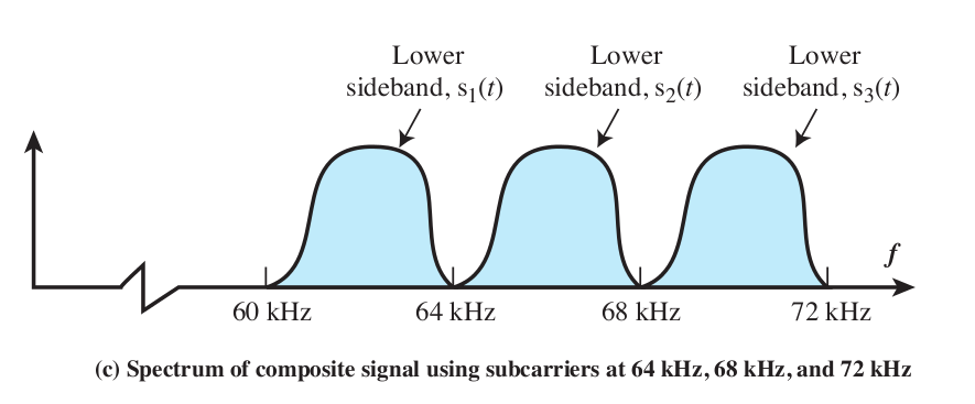
Brief comparison of Stallings Fig 5-8 (below) and Fig 8-5 (above).
Both show side-by-side bands, interfering minimally. The first is of two
bands in the voicerange (1 kHz and 2 kHz respectively), representing a modem
sending in opposite directions. The second is of multiple 4 kHz voice
bandsAM-modulated (using SSB) onto carriers of 60 kHz, 64 kHz, 68 kHz, ....