Asynchronous Transfer Mode
Peter Dordal, Loyola University CS Department
Asynchronous Transfer Mode, or ATM, is a packet-based
network model with excellent voice performance. The primary issues for voice
are
- small packets, to reduce fill time
- service guarantees, to minimize other network delays
ATM uses virtual-circuit switching and very small (53-byte) fixed-size
cells. The basic argument (mid-1980s) was that the virtual-circuit approach
is best when different applications have very different quality-of-service
demands (eg voice versus data). This is still a plausible argument, but
today's Internet is effectively very overbuilt and so VoIP data usually gets
excellent service even without guarantees.
The virtual-circuit argument makes an excellent point. Quality-of-service is
a huge issue in the IP internet. And many of the issues that led to IP over
ATM are more political than anything else. However, IP does make it
difficult to charge by the connection; this is not only a given with ATM,
but the telecommunications industry's backing would certainly lead one to
believe that telecom pricing would be in place. A DS0 line transfers about
480 KB/minute; today, a minute of long-distance is still often billed at
$0.05. That's 10 MB for a dollar, or a gigabyte for $100, or a typical 5 GB
monthly wireless-card cap for $500. That's a lot!
Why cells:
- reduces packetization (voice-fill) delay
- fixed size simplifies switch architecture
- lower store-and-forward delay
- reduces time waiting behind lower-priority big traffic
The ATM name can be compared to STM: what does the "A" really mean?
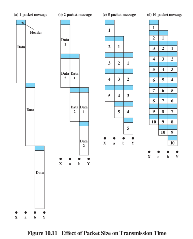
Review Stallings Fig 10.11 on large packets v small, and latency.
(Both sizes give equal throughput, given an appropriate window size.)

basic cellular issues
delay issues:
- 10 ms echo delay: 6 ms fill, ~4 ms for the rest
- In small countries using 32-byte ATM, the one-way echo delay might be
5 ms. Echo cancellation is not cheap!
Supposedly (see Peterson & Davie,
wikipedia.org/wiki/Asynchronous_Transfer_Mode) smaller countries wanted
32-byte ATM because the echo would be low enough that echo cancellation was
not needed. Larger countries wanted 64-byte ATM, for greater throughput. 48
was the compromise. (Search the WikiPedia article for "France".)
150 ms delay: threshhold for "turnaround delay" to be serious
packetization: 64kbps PCM rate, 8-16kbps compressed rate. Fill times: 6 ms,
24-48 ms respectively
buffering delay: keep buffer size >= 3-4 standard deviations, so buffer
underrun will almost never occur. This places a direct relationship between
buffering and jitter.
encoding delay: time to do sender-side compression; this can
be significant but usually is not.
voice trunking (using ATM links as trunks) versus voice switching (setting
up ATM connections between customers)
voice switching requires support for signaling
ATM levels:
- as a replacement for the Internet
- as a LAN link in the Internet
- MAE-East early adoption of ATM
- as a LAN + voice link in an office environment
A few words about how TCP congestion control works
- window size for single connections
- how tcp manages window size: Additive Increase / Multiplicative
Decrease (AIMD)
- Window size increases until queue overflows, causing packet loss
- queues are "normally full"
- congestion is in the hands of the end users
- TCP and fairness
- TCP and resource allocation
- TCP v VOIP traffic
ATM, on the other hand, avoids the "chaotic" TCP behavior (really chaotic IP
behavior) by dint of using virtual circuits. Virtual circuits put control of
congestion in the hands of the routers, and if a router cannot
guarantee you the service level you request then your connection will simply
not be completed (you can try later, or you can try with a lower-level
request; you may also be able to make requests well in advance).
VoIP is known for being cheaper, but also for having at least some negative
consequences for voice quality. There is such a thing as "Voice over ATM",
or VoATM, but you never hear about it because it is routine, of
identical quality to "Voice over T1" or "Voice over SONET".
VCC (Virtual Circuit Connection) and VPC (Virtual Path: bundle of VCCs)
Goal: allow support for QOS (eg cell loss ratio)
ATM cell format: Here it is in table format; the table is 8 bits wide:
Generic
flow control / VPI
|
Virtual
Path Identifier
|
VPI
|
Virtual Channel ID
|
| Virtual
Channel ID |
Virtual Channel ID
|
Payload Type, CLP bit
|
checksum
|
data (48
bytes)
|
The first 4 bits (labeled Generic Flow Control) are used for that only for
connections between the end user and the telecom provider; internally, the
first 12 bits are used for the Virtual Path Identifier. This is what
corresponds to the Virtual Circuit Identifier for VC routing.
The Virtual Channel Identifier is used by the customer to identify multiple
virtual paths to the same destination.
One point of having Virtual Channels is that later connections to the same
destination can be easily added, with no core-network involvement.
Internally, the core network can set up connections itself and use the
Virtual Channel Identifier however it wishes. The VPI/VCI separation also
reduces the number of connections the core network must manage.
3-bit PT (Payload Type) field:
- user bit
- congestion-experienced bit
- Service Data Unit (SDU) bit
CLP (Cell Loss Priority) bit: if we have congestion, is this in the first
group to be dropped, or the second?
The checksum is over only the 32 bits of the first four bytes of the header.
As such, it provides substantial error-correction
possibilities.
Header CRC; correction attempts; burst-error discards. One advantage of
having a checksum that covers only the header and not the data is that we
can make attempts to correct the error. A
straightforward if relatively time-consuming way to do this is to try
flipping each of the 40 header bits to see if this leads to a correct
checksum.
The GFC bits are sometimes used for signaling TRANSMIT, HALT/NO_HALT, spread
over time.
Transmission & synchronization
HUNT state; HEC field & threshhold for leaving, re-entering HUNT state
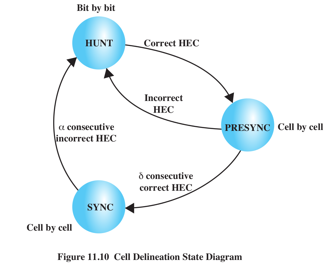
With a BER of 10-5, the probability of a corrupted 40-bit cell
header is about 4 × 10⁻⁴. If we take 𝛼=5, then the probability
of 𝛼 consecutive packets with a bad HEC field is about (4 × 10⁻⁴)5,
or 1 in 1017. We would send that many cells before a "false
positive" unsynchronization (that is, we thought we were unsynchronized, but
were not).
Once in the HUNT state, cell framing has failed, and so we check the HEC
every bit position; that is, for every bit position 0, we check if
bits 32-40 represent the CRC code for bits 0-31. If so, we have found a
correct HEC, and move to the PRESYNC state above. Of course, the HEC field
has only 8 bits, and so there is one chance in 256 that we have a correct
HEC field purely by accident. But if we take 𝛿=5, then the odds of a
correct HEC value by chance alone in 𝛿 consecutive packets is 1 in 2565
= 1012, and so we are reasonably sure that we are in fact
synchronized and move to the SYNC state. (A similar strategy is used to
synchronize SONET).
jitter and "depacketization delay"
The following diagram from Stallings shows how ATM packets are packed
end-to-end into an STM-1 payload envelope; the transport-overhead section of
the physical frame is not shown.
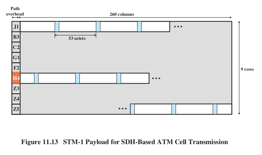
The Path Overhead H4 byte contains the offset (in bytes) to the start of the
first cell in the frame; it can range from 0 to 52. Of course, the entire
payload envelope can also float within the STM-1 physical frame.
_______________________________________________
ATM Delays, 10 switches and 1000 km at 155 Mbps
(from Walrand and Varaiya)
| cause |
time, in microsec |
reason
|
| Packetization delay |
6,000 |
48 bytes at 8 bytes/ms |
| propagation delay |
5,000 |
1000 km at 200 km/ms |
| transmission delay |
30 |
10 switches, 3microsec each at
155Mbps |
| queuing delay |
70 |
80% load => 2.4 cell avg queue, by
queuing theory; MeanCDT |
| processing delay |
280 |
28 microsec/switch |
| depacketization delay |
70++ |
worst-case queuing delay / MaxCDT |
AAL (ATM Adaptation Layers)
This is about the interface layer between the data (eg
bitstreams or packets) and the cells. Ultimately, this is how we chop up IP
packets and send them over ATM.
PDU: Protocol Data Unit, eg an IP packet from a higher level
CS-PDU: Convergence Sublayer PDU: how we "package" the user datagram to
prepare it for ATMification
A layout of the encapsulated user data (eg IP datagram), with ATM-specific
prefix & suffix fields added. See below under AAL3/4
SAR-PDU: Segmentation-and-Reassembly PDU; the "chopped-up" CS-PDU with some
cell-specific fields added
The first two layers are for specialized real-time traffic.
AAL 1 (sometimes known as AAL0)
constant-bit-rate source (voice/video)
AAL1 may include timestamps; otherwise buffering is used at receiver end.
This does include a three-bit (4-bit??) sequence number; payload is 47
bytes.
AAL 2
Intended for variable-bitrate real-time streams. The archetypal example is
voice/video subject to compression; video compression in particular tends to
compress by a different degree at different moments.
The next two layers are ways of dividing up IP packets, say, into cells. You
might wonder whether this is a good idea; traditionally, smaller packets
were associated with higher error rates. High error rates do encourage small
packets (so that only a small packet is lost/retransmitted when an error
occurs), and modern technology has certainly moved towards low error rates.
For a while, it was implicitly assumed that this also would mean large
packets.
But note that, for a (small) fixed bit
error rate, your overall error rate per KB will be about the same
whether you send it as a single packet or as ~20 ATM packets. The
probability of per-packet error will be roughly proportional to the size of
the packet. If the probability of a bit error in one 1000-byte packet is
1/10,000, then the probability of a bit error in one cell's worth, ~50
bytes, will be about 1 in 200,000, and the probability of a bit error in 20
cells (the original 1000-byte packet, now divided into cells), is 20 ×
1/20,000 = 1/1,000, the same as before. Dividing into ATM cells, in other
words, has no effect on the per-link bit error rate.
AAL 3/4
(Once upon a time there were separate AAL3 and AAL4 versions, but the
differences were inconsequential even to the ATM community.)
CS-PDU header & trailer:
CPI(8)
|
Btag(8)
|
BASize(16)
|
User data (big)
|
Pad
|
0(8)
|
Etag(8)
|
Len(16)
|
The Btag and Etag are equal; they help to detect the loss of the final cell
and thus two CS-PDUs run together.
BAsize = Buffer Allocation size, an upper bound on the actual size (which
might not yet be known).
The CS-PDU is frappéd into 44-byte chunks of user data (the SAR-PDUs)
preceded by type(2 bits) (eg first/last cell), SEQ(4), MID(10),
followed by length(6 bits), crc10(10 bits)
Type(2)
|
SEQ(4)
|
MID(10)
|
44-bye SAR-PDU
|
len(6)
|
crc10(10)
|
TYPE: 10 for first cell, 00 for middle cell, 01 for end cell, 11 for
single-cell message
SEQ: useful for detecting lost cells; we've got nothing else to help with
this!
MID: Multiplex ID; allows multiple streams
LEN: usually 44
AAL3/4: MID in SAR-PDU only (not in CS-PDU)
Note that the only error correction we have is a per-cell CRC10. Lost cells
can be detected by the SEQ field (unless we lose 16 cells in a row).
AAL 5
Somebody noticed AAL3/4, with 9 total header bytes for 44 data bytes, was
not too efficient. The following changes were made to create AAL 5. The main
"political" issue was to seize control of a single header bit, known at the
time as the "take back the bit" movement. This bit is used to mark the final
cell of each CS-PDU.
AAL-5 CS-PDU
Data (may be large)
|
pad
|
reserved(16)
|
len(16)
|
CRC32(32)
|
We then cut this into 48-byte
pieces, and put each piece into a cell. The last cell is marked.
The AAL 5 changes:
- Error checking moves from per-cell
CRC-10 to per-CS/PDU CRC-32
- An ATM header bit is used to
mark the last cell of a CS-PDU.
The header bit used to mark final cells is the SDU bit: 3rd bit of PT field.
Note that there is no ambiguity, provided we know that a given Virtual Path
or Virtual Channel is exclusively for AAL 3/4 traffic or exclusively for AAL
5 traffic.
The pad field means that every cell has a full 48 bytes of data
The last-cell header bit takes care of conveying the information in the AAL
3/4 Type field. The per-cell CRC(10) is replaced with per-CS/PDU CRC32.
What about the MID field? The observation is that we don't need it. We
seldom have multiple streams that need labeling with the MID, and if we do
we can always use additional virtual channels.
Why don't we need the SEQ field? Or the LEN field?
Why should ATM even support a standard way of encoding IP (or other) data?
Because this is really fragmentation/reassembly; having a uniform way to do
this is very helpful as it allows arbitrarily complex routing at the ATM
level, with reassembly at any destination.
Compare these AALs with header-encapsulation; eg adding an Ethernet header
to an IP packet
What about loss detection?
First, let us assume an error occurs that corrupts only 1 cell.
AAL3/4: The odds of checksum failure
are 1 in 210 (this is the probability that an error occurs but
fails to be detected).
AAL5: The odds of checksum failure are 1 in 232.
Now suppose we know an error corrupts two cells:
AAL3/4: failure odds: 1 in 220.
AAL5: failure odds: 1 in 232.
Errors in three cells: AAL5 still ahead!
Suppose there are 20 cells per CS-PDU. AAL3/4 devotes 200 bits to CRC; AAL5
devotes 32, and (if the error rate is low enough that we generally expect at
most three corrupted cells) still comes
out ahead.
Shacham & McKenney [1990] XOR technique: send 20-cell IP packet as 21
cells.
Last one is XOR of the others. This allows recovery from any one lost cell.
In practice, this is not necessary. It adds 5% overhead but saves a negligible
amount.
Also, dividing large IP packets into small cells means that, somewhere in
the network, higher-priority voice packets can be sent in
between IP-packet cells.
Another reason for ATM header error check: misaddressed packets mean the
right connection loses the packet, but also the wrong connection receives
the packet. That probably messes up reassembly on that second connection,
too.
ATM in Search of a Mission
How do you connect to your ISP?
How do you connect two widely separated LANs (eg wtc & lsc, or offices
in different states)
How do you connect five widely separated LANs?
Here are three general strategies:
- DS lines
- Frame Relay
- Carrier Ethernet (Metro Ethernet)
Method 1: lease DS1 (or fractional DS3) lines. This is expensive; these
lines are really intended as bundles of voice-grade lines, with very low
(sub-millisecond in some cases) delay guarantees. Why pay for that for bulk
data?
Method 2: lease Frame Relay connections.
The latter is considerably cheaper (50-70% of the cost)
DS1 has voice-grade capability built in. Delivery latency is tiny. You don't
need that for data.
What you do need is the DTE/DCE interface at each end.
DTE(you)---DCE - - - leased link - - - - DCE---DTE(you
again)
The red part here is under the control of the ISP; the black belongs to you.
Frame Relay: usually you buy a "guaranteed" rate, with the right to send
over that on an as-available basis.
"Guaranteed" rate is called CIR (committed information rate); frames may
still be dropped, but all non-committed frames will be dropped first.
Ideally, sum of CIRs on a given link is ≤ link capacity.
Fig 8e:10.19: frame-relay [LAPF] format; based on virtual-circuit switching.
(LAPB is a non-circuit-switched version very similar to HDLC, which we
looked at before when we considered sliding windows.)
Note DE bit: Basic rule is that everything you send over and above your CIR
gets the DE bit set.
Basic CS-PDU:
flag
|
VCI, etc
|
Data
|
CRC
|
flag
|
Extra header bits:
EA
|
Address field extension bit (controls
extended addressing) |
C/R
|
Command/response bit (for system
packets) |
FECN
|
Forward explicit congestion
notification |
BECN
|
Backward explicit congestion
notification |
D/C
|
address-bits control flag
|
DE
|
Discard eligibility |
(No sequence numbers!)
You get even greater savings if you allow the DE bit to be set on all
packets (in effect CIR=0).
(This is usually specified in your contract with your carrier, and then the
DE bit is set by their equipment).
This means they can throw your traffic away as needed. Sometimes minimum
service guarantees can still be worked out.
FECN and BECN allow packets to be marked
by the router if congestion is experienced. This allows
endpoint-based rate reduction. Of course, the router can only mark the FECN
packet; the receiving endpoint must take care to mark the BECN bit in
returning packets.
Bc and Be: committed and excess burst sizes; T =
measurement interval (CIR is in bytes/T; CIR = Bc/T).
Bc = T/CIR; however, the value of T makes a difference! Big T:
more burstiness.
Data rate r:
r ≤ Bc/T: guaranteed sending
Bc /T < r ≤ Be/T: as-available
sending
Be < r: do not send
Usually, Bc and Be (and T) are actually specified is
two token-bucket specifications, below. One problem with
our formulation here: do we use discrete averaging intervals of length T?
Another alternative: Carrier Ethernet service (sometimes
still called Metro Ethernet). Loyola uses (still?) this to connect LSC and
WTC.
Internally, traffic is probably carried on Frame Relay (or perhaps ATM)
circuits.
Externally (that is, at the interfaces), it looks like an Ethernet
connection. (Cable modems, DSL, non-wifi wireless also usually have
Ethernet-like interfaces.)
Here is the diagram from before, now showing Ethernet interfaces rather than
DTE-DCE. Again, the red is the ISP:
Network(you)---Ethernet jack - - - whatever they
see fit to use - - - - Ethernet jack---Network(you again)
This is the setting where ATM might still find a market. Its use is
"invisible", as a general way by which the carrier can send your data, over
their heterogeneous voice/data network, however is most convenient.
x.25 v frame relay (X.25 is obsolete)
real cost difference is that with the former, each router must keep packet
buffered until it is acknowledged
Token Bucket
Outline token-bucket algorithm, and leaky-bucket equivalent.
See http://intronetworks.cs.luc.edu/current/htmo/queuing.html#token-bucket-filters.
Token bucket as both a shaping and policing algorithm
- Bucket size b
- Entry rate r tokens/sec
packet needs to take 1 token to proceed, so long-term average rate is r
Bursts up to size b are allowed.
shaping: packets wait until their
token has accumulated.
policing: packets arriving with no token in bucket are dropped.
Both r and b can be fractional.
Fractional token arrival is possible: transmission fluid enters drop-by-drop
or continually, and packets need 1.0 units to be transmitted.
Leaky-bucket analog: Bucket size is still b, r = rate of leaking out.
A packet adds 1.0 unit of fluid to the bucket; packet is conformant
if the bucket does not overflow.
Token-bucket and leaky-bucket are two ways of describing the same
fundamental process: leaky bucket
means packets add to the bucket but are not allowed to overflow it;
transmission fluid leaks out with the passage of time. Token
bucket means that cells subtract from bucket; volume can't go
negative, transmission fluid is pumped into the bucket.
Leaky-bucket formulation is less-often used for packet management, but is
the more common formulation for self-repair algorithms:
faults are added to the bucket, and leak out over time. If the bucket is
nonempty for >= T, unit may be permanently marked "down"
HughesNet satellite-internet token-bucket (~2006):
- s = 350 MB
- r = 7 kBps (56kbps)
fill time: 50,000 sec ~ 14 hours
My current ISP has rh & rl (these were once 1.5
Mbit & 0.4 Mbit; they are now both higher).
I get:
rh / small_bucket interface layer
rl / 150 MB bucket
In practice, this means I can download at rh for 150 MB, then my
rate drops to rl.
While the actual limits are likely much higher in urban areas, more and more
ISPs are implementing something like this.
In general, if token-bucket (r,b) traffic arrives at a switch s, it can be
transmitted out on a link of bandwidth r without loss provided s has a queue
size of at least b.
In the ATM world, Token bucket is usually construed as a shaping algorithm:
note smoothing effect on big bursts, but ability to pass smaller bursts
intact.
Algorithm: tokens accumulate at a rate r, into a bucket with maximum
capacity D (=bucket depth). This is done by the token generator. The sender
needs to take a token out of the bucket (ie decrement the token count) each
time it sends a packet.
Token bucket with bucket size s=1, initially full, rate r=1/5
Conformant:
0 5 10 15 20 ...
0 6 11 16 21
NOT: 0 6 10 ...
NOT: 0 4 ...
We have a minimum of 5 time units between sending, and zero bucket capacity
beyond the one packet we want to send.
Token bucket with size s=1.2, initially full, rate r=1/5
This is now conformant:
0 6 10 16 20 ...
Here, we can save up 0.2 of a packet, so sometimes we can send after only 4
time units.
ATM Service categories
real-time:
CBR (Constant Bit Rate): voice & video; intended as ATM version of TDM
rt-VBR (real-time Variable Bit Rate): compressed voice/video; bursty
non-real-time:
nrt-VBR (non-real-time VBR): specify peak/ avg/burst in reservation
ABR (Available Bit Rate): subject to being asked to slow down
UBR (Unspecified Bit Rate): kind of like IP; only non-reservation-based
service
GFR (Guaranteed Frame Rate): better than UBR for IP; tries to optimize for
packet boundaries. If a cell has to be dropped, we might as well drop every
cell of the IP packet.
How do ABR, UBR, and GFR differ?
Traffic parameters describe the traffic
as it arrives at the network; that is, it describes the traffic we want
to send. Most important ones are in bold.
- peak cell rate
(PCR); actual rate may
momentarily exceed this due to randomization, related to CDV
- sustained cell rate (SCR)
- initial cell rate (ICR)
- cell delay variation tolerance (CDVT) (jitter tolerance); how
is this measured?
- burst tolerance (BT)
(essentially the bucket size; a measure of how bursty the traffic is)
- minimum cell rate (MCR)
CDVT is here because it describes what the application wants;
compare to CDV below.
The following QoS parameters describe what the network actually
delivers, in terms of losses and delays. These are not
about what the application wants, although an application may be very
interested in, say, MaxCTD.
- cell loss ratio (CLR)
- cell delay variation (CDV)
- peak-to-peak CDV
- Maximum cell transfer delay (MaxCTD)
- mean cell delay (MeanCTD)
- cell error ratio (unlike the others, this one is not subject to
negotiation)
Main ones are: PCR, , maxCTD, CDV, SCR, BT
Each service category above is defined by specifying the
traffic and QoS parameters as per the following table:
|
realtime |
non-realtime;
no delay requirements
|
| Attribute |
CBR |
rt-VBR |
nrt-VBR |
ABR |
UBR |
| CLR |
specified |
specified |
specified |
specified |
no |
CDV/CTD
MaxCTD
|
CDV +
maxCTD
|
CDV +
maxCTD
|
MeanCTD [?],
larger than for rt
|
no |
no |
| PCR, CDVT |
specified |
specified |
specified |
specified |
specified |
SCR, BT
|
N/A
|
specified
|
specified, larger
BT than rt-VBR
|
N/A
|
N/A
|
| MCR |
N/A
|
N/A
|
N/A
|
specified
|
N/A
|
Congestion
control
|
no
|
no
|
no
|
yes
|
no
|
[table from Walrand & Varaiya]
PCR: actual definition is sort of averaged over time; otherwise, two cells
sent back-to-back implies PCR of raw link bandwidth
Cell Delay Variation, and buffering : Fig 9e:13.6, 8e:13.8. Draw a vertical
line in the diagram to get list of packets currently in route (if the line
intersects D(i)) or in the receive buffer (if it intersects V(i)).
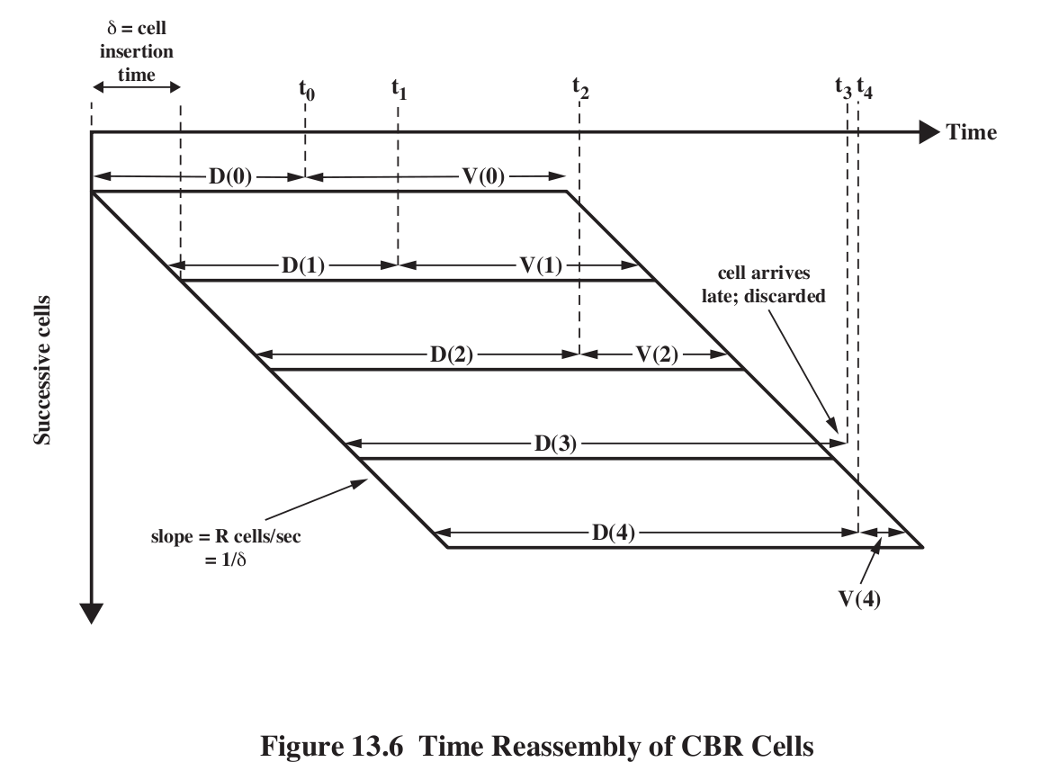
The first packet (packet 0) is sent at time T=0. Its propagation delay is
D(0). Upon arrival, the receiver holds it for an additional time V(0), to
accommodate possible fluctuations in future D(i). Packet transmission time
for the ith packet is k*i, where k is the packet sending interval (eg 6 ms
for 48-byte ATM cells). The ith packet arrives
at k*i + D(i). Let T be the time when we play back the first packet,
D(0)+V(0); this is the time between sending and playing. Then for each i,
D(i) +V(i) = T, so V(i) = T-D(i). Also, the ith packet needs to be played
back at T+k*i. A packet is late
(and thus unuseable) if D(i)>T.
V(0) is thus the value chosen for the initial receiver-side "playback
buffering time". If the receiver chooses too small a value, a larger
percentage of subsequent packets/cells may arrive too late. If V(0) is too
large, then too much delay has been introduced. Once V(0) is chosen, all the
subsequent V(i) are fixed, although there are algorithms to adapt T itself
up or down as necessary.
V(0) (or perhaps, more precisely, the mean value of all the V(i)) is also
known as the depacketization delay.
Suppose we know (from past experience with the network) the mean delay
meanD, and also the standard deviation
in D, which we'll call sd (more or less the same as CDV, though that might
be mean deviation rather than standard deviation). Assuming that we
believe the delay times are normally distributed, statistically, we can wait
three standard deviations and be sure that the packet will have arrived
99.99% of the time; if this is good enough, we can choose V(0) = meanD +
3*sd - D(0), which we might just simplify to 3*sd. If we want to use
CDV, statistical theory suggests that for the same 99.99% confidence we
might want to use 4*CDV. In general, we're likely to use something
like V(0) = k1 + k2*CDV.
Sometimes the D(i) are not
normally distributed. This can occur if switch queues are intermittently
full. However, that is more common in IP networks than voice-oriented
networks. On a well-behaved network, queuing theory puts a reasonable value
of well under 1 ms for this delay (Walrand calculates 0.07 ms).
Note that the receiver has no value for D(0), though it might have a pretty
good idea about meanD.
Note that the whole process depends on a good initial value V(0); this
determines the length of the playback
buffer.
V(n) is negative if cell n simply did not arrive in time.
For IP connections, the variation in arrival time can be hundreds of
milliseconds.
Computed arrival time; packets arriving late are discarded.
Note that
increased jitter
=> increased estimate for V(0)
=> increased overall delay!!!
ATM Congestion Management
The real strength of ATM is that it allows congestion-management mechanisms
that IP does not support. We'll look at some IP attempts below,
after ATM.
Last time we looked at ATM service categories. Traffic for each of these is
defined in terms of the Generalized Cell Rate Algorithm, below, a form of
Token-Bucket specification. An ATM system then has enough knowledge about
proposed connections to be able to decide whether to allow the connection or
not.
real-time:
CBR (Constant Bit Rate): voice & video; intended as ATM version of TDM
rt-VBR (real-time Variable Bit Rate): compressed voice/video; bursty
non-real-time:
nrt-VBR (non-real-time VBR): specify peak/ avg/burst in reservation
ABR (Available Bit Rate): subject to being asked to slow down
UBR (Unspecified Bit Rate): kind of like IP; only non-reservation-based
service
GFR (Guaranteed Frame Rate): better than UBR for IP; tries to optimize for
packet boundaries. If a cell has to be dropped, we might as well drop
every cell of the IP packet.
GCRA [generalized cell rate algorithm],
CAC [connection admission control]
CBR = rt-VBR with very low value for BT (token bucket depth)
rt-VBR: still specify maxCTD; typically BT is lower than for nrt-VBR
nrt-VBR: simulates a lightly loaded network; there may be bursts from other
users
Circuit setup involves negotiation of parameters
Routers generally do not try to control the individual endpoint sending
rates. Here are some things routers can
control:
- Admission Control (yes/no to connection)
- Negotiating lower values (eg lower SCR or BT) to a connection
- Path selection, internally
- Allocation of bandwidth and buffers to individual circuits/paths
- Reservations of bandwidth on particular links
- Selective dropping of (marked) low-priority cells
- ABR only: asks senders to slow down
- Policing
Congestion control mechanisms generally
- packet loss
- backpressure (good for x.25): a router sends slowdown indication to previous hop router
- choke packets (ICMP source quench): send slowdown to the source
- fast-retransmit: detect loss of packet N due to arrival of N+1, N+2,
and N+3 (sort of)
- monitoring of increasing RTT
- Explicit signaling - various forms
- DECbit style (or Explicit Congestion Notification)
- Frame Relay: FECN, BECN bits (latter is more common)
credit-based: aka window-based; eg TCP
rate-based: we adjust rate rather than window size
Note that making a bandwidth reservation may still entail considerable
per-packet delay!
Some issues:
- Fairness
- QoS
- Reservations
- priority queues
- multiple queues, "fair queuing"
- fair queuing and window size / queue usage
Priority queuing
http://intronetworks.cs.luc.edu/current/html/queuing.html#priority-queuing
The idea here is that a router has two (or more) separate queues: one for
high-priority traffic and one for low. When the router is ready to send a
packet, it always checks the high-priority queue first; if there is a packet
waiting there, it is sent. Only when the high-priority queue is empty is the
low-priority queue even checked.
Obviously, this means that if the high-priority queue always has some
packets, then the low-priority queue will "starve" and never get to send
anything. However, often this is not the case. Suppose, for example, that we
know that the total traffic in high-priority packets will never be more than
25% of the bandwidth. Then the remaining 75% of the bandwidth will
be used for low-priority traffic. Note that if the high-priority upstream
sender "empties the bucket" then for brief periods the router may send 100%
high-priority traffic.
Fair queuing
http://intronetworks.cs.luc.edu/current/html/queuing.html#fair-queuing
Suppose a router R has three pools of senders (perhaps corresponding to
three departments, or three customers), and wants to guarantee that each
pool gets 1/3 the total bandwidth. A classic FIFO router will fail at this:
if sender A does its best to keep R's queue full, while B and C are using
stop-and-wait and only send one packet at a time, then A will dominate the
queue and thus the bandwidth.
Fair Queuing addresses this by, in effect, giving each of A, B and C their
own queue. R then services these queues in round-robin fashion: one packet
from A, one packet from B, and one packet from C, and back to A. (There are
standard strategies for handling different-sized packets so as to guarantee
each sender the same rate in bytes/sec rather than in packets/sec, but we
can omit that for now.) Note that, if A's queue is full while B and C get
their next packet to R "just in time", then A now only gets 1/3 the total.
Note also that if sender C falls silent, then A and B now split the
bandwidth 50%-50%. Similarly, if B also stops sending then A will get 100%,
until such time as B or C resumes. That is, there is no "wasted" bandwidth
(as there would be with a time-division-multiplexing scheme).
Finally, if instead of equal shares you want to allocate 50% of the
bandwidth to A, 40% to B and 10% to C, the Fair Queuing scheme can be
adjusted to accommodate that.
In general, FIFO queues encourage senders to keep the queue as full as
possible. Any congestion-management scheme should take into account the kind
of behavior it is encouraging, and to avoid bad sender behavior. For
example, routers should discourage the user response of sending everything
twice (as might be the case if routers dropped every other packet).
ATM congestion issues:
- Real-time traffic is not amenable to flow control
- feedback is hard whenever propagation delays are significant
- bandwidth requirements vary over several orders of magnitude
- different traffic patterns and application loss tolerance levels
- latency/speed issues
Latency v Speed:
transmission time of a cell at 150 Mbps is about 3 microsec. RTT propagation
delay cross-country is about 50,000 microsec! We can have ~16,000 cells out
the door when we get word we're going too fast.
Note that there is no ATM sliding-windows mechanism!
ATM QoS agreements are usually for an entire Virtual Path, not
per-Virtual-Channel.
That is, the individual channels all get one lump QoS, and the endpoints are
responsible for fairness among the VCCs
Traffic policing v shaping (essentially provider-based v sender-based)
Generalized Cell Rate Algorithm, GCRA
http://intronetworks.cs.luc.edu/current/html/queuing.html#gcra
The GCRA is an alterative formulation of Token Bucket.
GCRA(T,𝝉): T = average time between packets, 𝝉 = tau = variation
We define "theoretical arrival time", or tat, for each cell, based on the
arrival time of the previous cell.
Cells can always arrive later, but not earlier.
Arriving late doesn't buy the sender any "credit", though (in this sense,
the bucket is "full")
Initially tat = current clock value, eg tat=0.
Suppose the current cell is expected at time tat, and the expected cell
spacing is T.
Let t = actual arrival time
Case 1: t < tat - 𝝉 (the cell arrived too EARLY)
- mark cell as NONCONFORMING
- do not change tat (applies to next cell)
Case 2: t >= tat - 𝝉
- cell is CONFORMING
- newtat = max(t,tat) + T
draw picture of t<tat−𝝉, tat−𝝉<= t < tat and tat < t. The last
case is "late"
Examples: GRCA(10,3) for the following inputs
0, 10, 20, 30
0, 7, 20, 30
0, 13, 20, 30
0, 14, 20, 30
1, 6, 8, 19, 27
CGRA(3,12):
arrivals: 0,0,0,0, 0, 3, 9,10,15
tats: 0,3,6,9,12,15,18,21,24
What is "fastest" GCRA(3,16) sequence?
peak queue length is approx 𝝉/T
better: 𝝉/(T-1) + 1
Token bucket: accumulate "fluid" at rate of 1 unit per time unit.
Bucket capacity: T+𝝉; need T units to go (or (T+𝝉)/T, need 1 unit)
A packet arriving when bucket contents >= T is conformant.
Conformant response: decrement bucket contents by T.
Nonconformant response: do nothing (but maybe mark packets)
Token bucket formulation of GCRA:
- bucket size T+𝝉
- bucket must contain T units at cell arrival time
- No: nonconformant
- Yes: take out T units
Cell Loss Priority bit
An ATM router can mark a cell's CLP bit (that is, set it to CLP=1) if the
cell fails to be compliant for some ingress token-bucket specification. Some
further-downstream router then may decide it needs to drop CLP=1 packets to
avert congestion, meaning that the marked traffic is lost. However, it is
also possible that the marked traffic will be delivered successfully.
The sender will likely negotiate a traffic specification for both CLP=0
traffic. It may also, separately and optionally, negotiate terms for CLP=0
and CLP=1 traffic together; this latter is the CLP-0-or-1 contract.
Of course, the sender cannot be sure this traffic won't be dropped; it is
carried by the network only on a space-available basis. In this situation,
the agreement would likely allow the network to set CLP=1 for nonconforming
traffic on entry.
Another option is for the carrier to allow the sender to set CLP; in this
case, the contract would cover CLP=0 cells only. Noncompliant CLP=0 traffic
would be dropped immediately (thus providing an incentive for the sender not
to mark everything CLP=0), but the sender could send as much CLP=1 traffic
as it wanted.
Suppose a user has one contract for CLP=0 traffic and another for CLP-0-or-1
traffic. Here is a plausible strategy, where "compliant" means compliant
with all token-bucket policing (see the GCRA algorithm below for details).
cell
|
compliance
|
action
|
CLP = 0
|
compliant for CLP = 0
|
transmit
|
CLP = 0
|
noncompliant for CLP=0 but compliant
for CLP-0-or-1 |
set CLP=1, transmit
|
CLP = 0
|
noncompliant for CLP=0 and
CLP-0-or-1 |
drop
|
CLP = 1
|
compilant for CLP-0-or-1 |
transmit
|
CLP = 1
|
noncompliant for CLP-0-or-1 |
drop
|
A big part of GFR is to make sure that all the cells of one larger IP frame
have the same CLP mark, on entry. A subscriber is assigned a guaranteed
rate, and cells that meet this rate are assigned a CLP of 0. Cells of
additional frames are assigned CLP = 1.
ATM routers might not want to reorder traffic; ATM in general frowns upon
reordering. However, if reordering were permitted, a router could use
priority queuing to forward CLP=0 packets at high priority and CLP=1 packets
at low priority.
CLP bit and conformant/nonconformant
ATM Traffic Specification
Here we specify just what exactly the ATM service categories are,
in terms of token bucket (actually GCRA).
CBR traffic
1. Specify PCR and CDVT. We will assume PCR is represented as cells per cell
transmission time.
2. meet GCRA(1/PCR, CDVT)
What does this mean?
6 ms sending rate, 3 ms CDVT
cells can be delayed by at most CDVT!
VBR traffic (both realtime and nrt)
GCRA(1/PCR, CDVT) and
GCRA(1/SCR, BT+CDVT)
Note CDVT can be zero!
What does big 𝝉 do?
Example: PCR = 1 cell/microsec
SCR = 0.2 cell/microsec
CDVT = 2 microsec
BT = 1000 cells at 0.2 cell/microsec = 200 microsec
GCRA(1,2): delay cells by at most 2 microsec
GCRA(5,200): would have allowed delay of 200 microsec, but disallowed by
first.
Allow 0 1 2 3 ... 999 5000
rt versus nrt traffic: Generally the latter has larger BT values (as well as
not being allowed to specify maxCTD, and generally having a much larger
value for meanCTD).
For both CBR and VBR traffic, the sender may negotiate separate values for
CLP 0 and CLP 0+1 traffic.
Traffic Shaping
ATM VBR-class traffic can be shaped,
say by emitting cells at intervals of time T.
This works for nrt-VBR, but will break CTD bound for rt-VBR
Example:
CGRA(3,12):
arrivals: 0,0,0,0, 0, 3, 9,10,15
tats: 0,3,6,9,12,15,18,21,24
GCRA(1,2) & GCRA(5,200):
These are traffic descriptions; the
network only makes loss/delay promises
GCRA(1,2): At the PCR of 1/1, cells can be early by at most 2
GCRA(5,200): At SCR of 1/5, cells can be early by 200.
But the 200 cells cannot arrive faster than PCR, by more than 2
ABR: available bit rate
UBR: unspecified bit rate
GFR: Guaranteed Frame Rate
For ABR, the network offers the PCR, subject to being >= the MCR. The
network can move PCR up and down.
For UBR, the user specifies the PCR and the CDVT.
ATM Admission Control
Because this is telecom, the most important thing is to keep the CBR traffic
flowing with no more delay than propagation delay, basically.
ATM routers need to decide when they can accept another connection.
(Often the issue is whether to accept a new circuit, or VCC, on an aggregate
path, or VPC. Often VPCs are under the same administrative jurisdiction as
all the component VCCs.)
CAC = connection admission control.
Note that policing, or determining
if a connection stays within its contracted parameters, is an entirely
different issue.
UBR: all that matters is if PCR
<= free_bandwidth; in this setting, we don't necessarily use bucket sizes
at all. Note that not all of existing allocated bandwidth may be used. We
use a priority queue, and have UBR traffic be the lowest priority. This
amounts to the requirement that sum(PCR) <= free_bandwidth for all UBR
connections.
Actually, if sum(PCR) == free_bandwidth, we can be in a bit of a fix as to
analyzing peaks. Figuring out how statistics can help us out here is tricky;
getting a good handle on the statistical distribution of data-transmission
bursts is not trivial.
ABR: this traffic depends on "space available"
ABR v UBR: ABR gets guaranteed service bounds if
it abides by the rules
ABR senders receive the ACR: (allowed cell rate) from their router; they
also use also Minimum/Peak/Initial CR
significance of MCR (minimum cell rate)
ABR uses RM (resource manager) cells, that circulate over ABR paths and help
the sender measure the available bandwidth.
RM cells are sent periodically over the link. They include a requested
rate, for future data cells. They also contain the following bits:
- Congestion Indicated (CI) bit
- No Increase (NI) bit
- Explicit Cell Rate Field (ER)
CI indicates more serious congestion than NI.
CI set: reduce ACR by a percentage
CI not set, NI not set: increase ACR by percentage
CBR: reserve bandwidth, handle these queues on round-robin/fair-queuing
basis
VBR
Suppose our bandwidth cap is C. We can require sum(PCR) <= C, or sum(SCR)
<= C. Both work, but note that the total queue size needed will be
approximately the sum of the appropriate Burst Tolerances (BTs). A VBR flow
will typically meet GCRA(1/PCR, BT1) and GCRA(1/SCR, BT2), where the BT2 is
much higher than BT1. Therefore,
the worst-case queue backlog (representing delay)
will be much worse for sum(SCR) = C than for sum(PCR) = C.
How many GCRA(T,𝝉) flows can we have? 1/T = SCR
nrt-VBR: to support a GCRA(T1,𝜏1)
flow, need 𝜏1/T1 +1 buffer space. (Actually buffer
space ~ 𝜏1/(T1-1) + 1)
To support that and GCRA(T2,𝜏2), we need:
- total available rate >= 1/T1 + 1/T2
- buffer space >= total buffer space for each
rt-VBR and CTD
For nrt-VBR, all that is needed to meet a traffic specification GCRA(T,𝝉)
is a bandwidth in excess of 1/T, and sufficient queue size to hold a burst.
For rt-VBR, by comparison, we need to take maxCDT into account too. This
makes things just a little more complicated, because a simple rule such as
sum(SCR)≤C may still leave us with queues that we have the bandwidth and
buffer space to handle, but not in enough
time to meed the maxCTD requirement.
Here is an analysis that attempts to take this maxCTD requirement into
account. It is from Walrand & Varaiya, High-Performance Communications
Networks, Admission Control, 2e:p 398.
See also http://intronetworks.cs.luc.edu/current/html/queuing.html#delay-constraints
The first step is to calculate the maximum queue (cell backlog). We approach
this by trying to figure out the "worst case". The analysis here basically
establishes that a GCRA(T,𝝉) flow will have a maximum queue utilization of
floor(𝜏/(T-1)) + 1, assuming the outbound rate is at least 1/T.
Step 1: given GCRA(T,𝝉), what is the "fastest sequence" of cell times?
In such a fastest sequence, we will always have t = tat - 𝜏: ; newtat =
max(tat) + T
GCRA(5, 2): 0 3 8 13 18 23...
GCRA(5,10):
arrivals
|
0
|
0
|
0
|
5
|
10
|
15
|
20
|
tats
|
0
|
5
|
10
|
15
|
20
|
25
|
30
|
In every case, (tat - arrival) <=10, and = 10 when possible
Graph of GCRA(3,25), output line rate = 2.5 ticks per cell
(C = 0.4 cells/tick)
Fastest when we allow multiple cells at the same time tick:
0 0 0 0 0 0 0
0 0 2 5
Fastest when we need 1 tick for each cell:
0
1 2 3 4 5 6 7 8 9 10 11 12
14 17 20
tats: 0
3 6 9 12 15 18 21 24 27 30 33 36 39 42 45
peak backlog: 8 cells / 13 cells
13 = floor(𝝉/(T-1))+1 = floor(25/2)+1
Now we need to decide the bandwidth actually needed to accept an rt-VBR
connection satisfying GCRA(T,𝜏), and with a delay constraint. For a single
flow, define M = MaxQueue = floor(𝜏/(T-1)) + 1
Let D = max delay (in cell
transmission times) at this particular switch; the total delay through K
switches might be DK.
C = bandwidth of the outbound link.
What is requirement on bandwidth to handle one
connection?
We need C ≥ M/D, where M/D = rate needed to send queue M in time D
[If we're not concerned about D, all we need is enough bandwidth to stay
ahead in the long run, and enough buffer space to handle worst-case M, and
we can make cell-loss guarantees.]
Also need C > 1/T, the nominal bandwidth; these two constraints can be
combined into
C ≥ max(1/T, M/D)
When does the second term here dominate? That is, when is
M/D > 1/T? Another way to write this is D < TM. TM = time to send a
burst, at the existing rate
With N connections, we get something like
effective bandwidth needed = N * max(1/T, M/D)
Max backlog is NM; need this cleared in time D so NM <= CD.
C ≥ N×(M/D)
Also need C≥N/T, so this yields
C≥ N × max(1/T, M/D)
as above
For D small, meaning the M/D term dominates, α := max(1/T, M/D)
is M/D; about D/M connections can be accommodated
Let us measure D in units of inter-cell spacing.
T measured by those units is 1.
Note D<<T is certainly a possible
requirement.
Question: when is 1/T < M/D? (so M/D term dominates)
ie T > D/M?
ie D < TM?
Now take T=1. If D<M, we need extra bandwidth allocation to handle delay.
If D>M, then we can take care of a backlog of M simply by sending at the
advertised PCR, and no special delay guarantee is needed.
Need extra bandwidth if D < M, and we thus cannot get rid of a burst
using usual PCR.
Recall D = max delay, M = time needed to process a burst
Example 1: Suppose we have a GCRA(3,18) flow, with times
measured in µsec, and D=40 µsec. By our formula above, M=floor(18/2) + 1 =
10. M/D is thus 40 /10 = 4 µsec/cell. The rate needed to keep up with the
steady-state case, however, is 1/T = 3 µsec/cell; the bandwidth needed is
1/3 cells/µsec.
Example 2: Now suppose in the previous example that the
delay constraint D falls to 20 µsec. M/D is now 2 µsec/cell, and the
bandwidth needed is 1/2 cells/µsec. This is 50% more than the bandwidth of
1/3 cells/µsec needed to keep up with the steady-state case.
Video example
video connections: 2 Mbps average, peak 10 Mbps (for active scenes)
peak bursts last up to 10 sec, D = 0.1 sec
Burst: 10Mbps for 10 sec = 100 Mbit = 12 MB = 250 K cells
suppose we have 200Mbps = 471 cells/ms
Do we assign 100 connections, using average? or 20, using peak?
Line rate: 10 Mbps = PCR = 23 cells/ms
max back-to-back cells: 10 sec worth, M = 230,000 cells
Acceptable delay = 10 ms = 2300 cells
α = max(1/T, M/(D+M-1)) = M/(D+M-1) ~ 1.0; must treat as at line rate
statistical approach might double this, if we make the assumption that busy
times are, say, 10% of total.
ATM Summary
- GCRA(T,𝝉) can be used to define traffic specifications
- For one (or more!) GCRA specs, we can define a fastest
sequence (ie fastest compliant arrival times)
- GCRA can be used (often in pairs) to specify the ATM service
categories and their specific needs
- Given a bottleneck link, we can use the GCRA parameters T and 𝝉 to
compute the maximum burst queue
- To get a bound on MaxCTD (MaxDelay), we need bandwidth ≥ PCR, but also
(and this is usually the more significant limitation) sufficient
bandwidth to clear any burst queue within the time constraint allotted
The latter applies to the IP world as well. Suppose we want a hard bound T
on total delay along a path through N routers. We first have to subtract the
propagation delay TP to get the max queuing delay TQ =
T - TP. Then we get the per-router time TR by dividing
TP by N: TR = TP/N (equal division is not
essential). Then, each router must guarantee, given its outbound bandwidth
and its inbound bandwidth(s) and bucket sizes (burst tolerances), that a
worst-case burst can be cleared in time TR.