Comp 346/488: Intro to Telecommunications
Tuesdays 4:15-6:45, Lewis Towers 412
Class 12, Apr 10
Chapter 11, ATM
Chapter 13, congestion control (despite the title, essentially all the detailed information is ATM-specific)
Chapter 14, cellular telephony
Asterisk questions
ATM
The basic argument (mid-1980s): Virtual circuit approach is best when
different applications have very different quality-of-service demands
(eg voice versus data).
This argument makes an excellent point. Quality-of-service is a huge
issue in the IP internet. And many of the issues that led to IP over
ATM are more political than anything else. However, IP does make it
difficult to charge by the connection; this is not only a given with
ATM, but the telecommunications industry's backing would certainly lead
one to believe that telecom pricing would be in place.
A DS0 line transfers about 480KB/minute; today, a minute of
long-distance goes for about $0.05. Thats 10 MB for a dollar, or a
gigabyte for $100, or a typical 5 GB monthly wireless-card cap for $500.
VCC (Virtual Circuit Connection) and VPC (Virtual Path: bundle of VCCs)
Goal: allow support for QOS (eg cell loss ratio)
ATM cell format: Fig 11.6 (9th ed.), 11.4 (7th & 8th eds). Here it is in table format; the table is 8 bits wide:
Generic flow control / VPI
|
Virtual Path Identifier
|
VPI
|
Virtual Channel ID
|
| Virtual Channel ID
|
Virtual Channel ID
|
Payload Type, CLP bit
|
checksum
|
data (48 bytes)
|
The first 4 bits (labeled Generic Flow Control) are used for that
only for connections between the end user and the telecom provider;
internally, the first 12 bits are used for the Virtual Path Identifier.
This is what corresponds to the Virtual Circuit Identifier for VC
routing.
The Virtual Channel Identifier is used by the customer to identify multiple virtual paths to the same destination.
One point of having Virtual Channels is that later connections to
the
same destination can be easily added, with no core-network involvement.
Internally, the core network can set up connections itself and use the
Virtual Channel Identifier however it wishes. The VPI/VCI separation
also reduces the number of connections the core network must manage.
3-bit PT (Payload Type) field: user bit, congestion-experienced bit, Service Data Unit (SDU) bit
CLP (Cell Loss Priority) bit: if we have congestion, is this in the
first group to be dropped, or the second?
The checksum is over only the 32 bits of the first four bytes of the header. As such, it provides substantial error-correction possibilities.
Header CRC; correction attempts; burst-error discards
why protect the header?
Error-correcting options; fig 9e:11.8, 8/7e:11.6)
GFC field: TRANSMIT, HALT/NO_HALT (spread over time)
Transmission & synchronization
HUNT state; HEC field & threshhold for leaving, re-entering HUNT state; this is illustrated in 9e:fig11.10.
More on synchronization process, α and δ values (Fig 9e:11.11 (α=5,7,9), Fig 9e:11.12 (δ=4,6,8))
jitter and "depacketization delay"
STM-1 diagram, Fig 9e:11.13, 7/8e:11.11: note use of H4 to contain offset to the start of the first cell in the frame.
Perspective of ATM as a form of TDM; note 87*3 = 261 columns, minus 1 for path overhead
_______________________________________________
ATM Delays, 10 switches and 1000 km at 155 Mbps
(from Walrand?)
| cause |
time, in microsec |
reason
|
|
Packetization delay |
6,000 |
48 bytes at 8 bytes/ms |
|
propagation delay |
5,000 |
1000 km at 200 km/ms |
|
transmission
delay |
30 |
10 switches, 3microsec each at 155Mbps |
|
queuing
delay |
70 |
80% load => 2.4 cell avg queue, by queuing theory; MeanCDT |
|
processing
delay |
280 |
28 microsec/switch |
|
depacketization delay |
70++ |
worst-case queuing delay /
MaxCDT |
AAL (ATM Adaptation Layers)
(not really in Stallings)
This is about the interface layer between the data (eg bitstreams or packets) and the cells
PDU: Protocol Data Unit, eg an IP packet from a higher level
CS-PDU: Convergence Sublayer PDU: how we "package" the user datagram to prepare it for ATMification
A layout of the encapsulated user data (eg IP datagram), with
ATM-specific prefix & suffix fields added. See below under AAL3/4
SAR-PDU: Segmentation-and-Reassembly PDU; the "chopped-up" CS-PDU with some cell-specific fields added
AAL 1 (sometimes known as AAL0)
constant-bit-rate source (voice/video)
AAL1 may include timestamps; otherwise buffering is used at receiver end.
This does include a three-bit (4-bit??) sequence number; payload is 47 bytes.
AAL 2
Intended for analog streams (voice/video subject to compression, thus having a variable bitrate)
AAL 3/4
(Once upon a time there were separate AAL3 and AAL4
versions, but the differences were inconsequential even to the ATM
community.)
CS-PDU header & trailer:
CPI(8)
|
Btag(8)
|
BASize(16)
|
User data (big)
|
Pad
|
0(8)
|
Etag(8)
|
Len(16)
|
The Btag and Etag are equal; they help to detect the loss of the final cell and thus two CS-PDUs run together.
BAsize = Buffer Allocation size, an upper bound on the actual size (which might not yet be known).
The CS-PDU is frappéd into 44-byte chunks of user data (the SAR-PDUs)
preceded by type(2 bits) (eg first/last cell), SEQ(4), MID(10),
followed by length(6 bits), crc10(10 bits)
Type(2)
|
SEQ(4)
|
MID(10)
|
44-bye SAR-PDU
|
len(6)
|
crc10(10)
|
TYPE: 10 for first cell, 00 for middle cell, 01 for end cell, 11 for single-cell message
SEQ: useful for detecting lost cells; we've got nothing else to help with this!
MID: Multiplex ID; allows multiple streams
LEN: usually 44
AAL3/4: MID in SAR-PDU only (not in CS-PDU)
Note that the
only error correction we have is a per-cell CRC10. Lost cells can be
detected by the SEQ field (unless we lose 16 cells in a row).
Note also that if the bit error rate is constant, the packet error rate is about the same whether you send the packet as one big unit or as a bunch of small cells.
AAL 5
Somebody noticed AAL3/4 was not too efficient. The following changes were made
CS-PDU
Data (may be large)
|
pad
|
reserved(16)
|
len(16)
|
CRC32(32)
|
We then cut this into 48-byte pieces, and put each piece into a cell. The last cell bears the "header mark".
-
Move error checking from per-cell CRC-10 to per-CS/PDU CRC-32
-
use ATM header bits to mark last cell; AAL5 launched the "take back the bit" movement
-
use SDU bit: 3rd bit of PT field
- The pad field means that every cell has a full 48 bytes of data
The last-cell header bit takes care of the AAL 3/4 Type field. The per-cell CRC(10) is replaced with per-CSPDU CRC32.
What about the MID field? We don't even need it!
Why don't we need the SEQ field? Or the LEN field?
Why should ATM even support a standard way of encoding IP (or other)
data? Because this is really fragmentation/reassembly; having a uniform
way to do this is very helpful as it allows arbitrarily complex routing
at the ATM level, with reassembly at any destination.
Compare these AALs with header-encapsulation; eg adding an Ethernet header to an IP packet
What about loss detection?
Assuming a local error that corrupts only 1 cell,
AAL3/4: The odds of checksum failure are 1 in 210 (this is the probability that an error occurs but fails to be detected).
AAL5: The odds of checksum failure are 1 in 232.
Errors in two cells:
AAL3/4: failure odds: 1 in 220.
AAL5: failure odds: 1 in 232.
Errors in three cells: AAL5 still ahead!
Suppose there are 20 cells per CS-PDU. AAL3/4 devotes 200 bits to CRC; AAL5
devotes 32, and (if the error rate is low enough that we generally
expect at most three corrupted cells) still comes out ahead.
Shacham & McKenney [1990] XOR technique: send 20-cell IP packet as 21 cells.
Last one is XOR of the others. This allows recovery from any one lost
cell. In practice, this is not necessary. It adds 5% overhead but saves
a negligible amount.
High error rates encourage small packets (so that only a small packet
is lost/retransmitted when an error occurs). Modern technology moves
towards low error rates. For a while, it was implicitly assumed that
this also would mean large packets. But note that, for a (small) fixed bit error rate,
your overall error rate per KB will be about the same whether you send
it as a single packet or as ~20 ATM packets. The probability of
per-packet error will be roughly proportional to the size of the packet.
Also, dividing large IP packets into small cells means that, somewhere
in the network, higher-priority voice packets can be sent in between IP-packet cells.
Another reason for ATM header error check: misaddressed packets mean
the right connection loses the packet, but also the wrong connection receives the packet. That probably messes up reassembly on that second connection, too.
Carrier Ethernet (Metro Ethernet) service v Frame Relay v DS lines
How do you connect to your ISP?
How do you connect two widely separated LANs (eg wtc & lsc, or offices in different states)
How do you connect five widely separated LANs?
Method 1: lease DS1 (or fractional DS3) lines.
Method 2: lease Frame Relay connections.
The latter is considerably cheaper (50-70% of the cost)
DS1 has voice-grade capability built in. Delivery latency is tiny. You don't need that for data.
What you do need is the DTE/DCE interface at each end.
DTE(you)---DCE - - - leased link - - - - DCE---DTE(you again)
Frame Relay: usually you buy a "guaranteed" rate, with the right to send over that on an as-available basis.
"Guaranteed" rate is called CIR (committed information rate); frames
may still be dropped, but all non-committed frames will be dropped
first.
Ideally, sum of CIRs on a given link is ≤ link capacity.
Fig 8e:10.19: frame-relay [LAPF] format; based on virtual-circuit
switching. (LAPB is a non-circuit-switched version very similar to
HDLC, which we looked at before when we considered sliding windows.)
Note DE bit: Basic rule is that everything you send over and above your CIR gets the DE bit set.
Basic CS-PDU:
flag
|
VCI, etc
|
Data
|
CRC
|
flag
|
Extra header bits:
EA
|
Address field extension bit (controls extended addressing) |
C/R
|
Command/response bit (for system packets) |
FECN
|
Forward explicit congestion notification |
BECN
|
Backward explicit congestion notification |
D/C
|
address-bits control flag
|
DE
|
Discard eligibility |
(No sequence numbers!)
You get even greater savings if you allow the DE bit to be set on all packets (in effect CIR=0).
(This is usually specified in your contract with your carrier, and then the DE bit is set by their equipment).
This means they can throw your traffic away as needed. Sometimes minimum service guarantees can still be worked out.
FECN and BECN allow packets to be marked by the router
if congestion is experienced. This allows endpoint-based rate
reduction. Of course, the router can only mark the FECN packet; the
receiving endpoint must take care to mark the BECN bit in returning
packets.
Bc and Be: committed and excess burst sizes; T = measurement interval (CIR is in bytes/T; CIR = Bc/T).
Bc = T/CIR; however, the value of T makes a difference! Big T: more burstiness
Data rate r:
r < Bc: guaranteed sending
Bc < r < Be: as-available sending
Be < r: do not send
One problem: do we use discrete averaging intervals of length T?
Another alternative: Carrier Ethernet service (sometimes still called
Metro Ethernet). Loyola uses (still?) this to connect LSC and WTC.
Internally, traffic is probably carried on Frame Relay (or perhaps ATM) circuits.
Externally
(that is, at the interfaces), it looks like an Ethernet connection.
(Cable modems, DSL, non-wifi wireless also usually have Ethernet-like
interfaces.)
This is the setting where ATM might still find a market.
x.25 v frame relay:
real cost difference is that with the former, each router must keep packet buffered until it is acknowledged
Congestion and Traffic Management
A few words about how TCP congestion control works
- window size for single connections
- how tcp manages window size: Additive Increase / Multiplicative
Decrease (AIMD)
- TCP and fairness
- TCP and resource allocation
- TCP v VOIP traffic
Brief discussion of TCP congestion management
- congestion window
- additive-increase, multiplicative decrease
- windows with no loss: cwnd += 1
- windows experiencing loss: cwnd = cwnd/2
This tends to oscillate between a full queue at the bottleneck router,
and half that (including packets in transit). Sometimes this leads to
considerable unnecessary delay.
Token Bucket
Outline token-bucket algorithm, and leaky-bucket equivalent.
Token bucket as both a shaping and policing algorithm
See Fig 9e:13.9 (78e:13.11)
-
Bucket size b
-
Entry rate r tokens/sec
packet needs to take 1 token to proceed, so long-term average rate is r
Bursts up to size b are allowed.
shaping: packets wait until their token has accumulated.
policing: packets arriving with no token in bucket are dropped.
Both r and b can be fractional.
Fractional token arrival is possible: transmission fluid enters drop-by-drop or continually, and packets need 1.0 cups to go.
Leaky-bucket analog: Bucket size is still b, r = rate of leaking out.
A packet adds 1.0 unit of fluid to the bucket; packet is conformant if the bucket does not overflow.
Leaky-bucket formulation is less-often used for packet management,
but is the more common formulation for self-repair algorithms:
faults are added to the bucket, and leak out over time. If the bucket
is nonempty for >= T, unit may be permanently marked "down"
HughesNet satellite-internet token-bucket (~2006):
-
s = 350 MB
-
r = 7 kBps (56kbps)
fill time: 50,000 sec ~ 14 hours
My current ISP has rh & rl (1.5 Mbit & 0.4 Mbit??).
I get:
rh / small_bucket
rl / 150 MB bucket
In practice, this means I can download at rh for 150 MB, then my rate drops to rl.
While the actual limits are likely much higher in urban areas, more and more ISPs are implementing something like this.
In general, if token-bucket (r,b) traffic arrives at a switch s, it can
be transmitted out on a link of bandwidth r without loss provided s has
a queue size of at least b.
ATM Service categories
realtime:
CBR: voice & video; intended as ATM version of TDM
rt-VBR: compressed voice/video; bursty
nonrealtime:
nrt-VBR: specify peak/ avg/burst in reservation
ABR: subject to being asked to slow down
UBR: kind of like IP; only non-reservation-based service
GFR: guaranteed frame rate: better than UBR for IP; tries to optimize for packet boundaries
How do ABR, UBR, and GFR differ?
traffic parameters (these describe what we want to send). Most important ones are in bold.
-
peak cell rate (PCR); actual rate may exceed this due to randomization, related to CDV
- sustained cell rate (SCR)
-
initial cell rate (ICR)
-
cell delay variation tolerance (CDVT) (jitter tolerance); how is this measured?
-
burst tolerance (BT) (a measure of how bursty the traffic is)
-
minimum cell rate (MCR)
statistics
leaky buckets & token-bucket depth
QoS parameters (these describe losses and delays):
-
cell loss ratio (CLR)
-
cell delay variation (CDV)
-
peak-to-peak CDV
- Maximum cell transfer delay (MaxCTD)
- mean cell delay (MeanCTD)
- cell error ratio (unlike the others, this one is not subject to negotiation)
Main ones are: PCR, CDV, SCR, BT (summarized in table 9e:13.2)
Characteristics:
|
realtime |
non-realtime; no delay requirements
|
| Attribute |
CBR |
rt-VBR |
nrt-VBR |
ABR |
UBR |
|
CLR |
specified |
specified |
specified |
specified |
no |
CDV/CTD
MaxCTD
|
CDV +
maxCTD
|
CDV +
maxCTD
|
MeanCTD [?],
larger than for rt
|
no |
no |
|
PCR, CDVT |
specified |
specified |
specified |
specified |
specified |
SCR, BT
|
N/A
|
specified
|
specified, larger
BT than rt-VBR
|
N/A
|
N/A
|
| MCR |
N/A
|
N/A
|
N/A
|
specified
|
N/A
|
Congestion
control
|
no
|
no
|
no
|
yes
|
no
|
[table from Walrand & Varaiya]
PCR: actual definition is sort of averaged over time; otherwise, two cells sent back-to-back implies PCR of raw link bandwidth
Cell Delay Variation, and buffering : Fig 9e:13.6, 8e:13.8.
Draw a vertical line in the diagram to get list of packets currently in
route (if the line intersects D(i)) or in the receive buffer (if it
intersects V(i)).
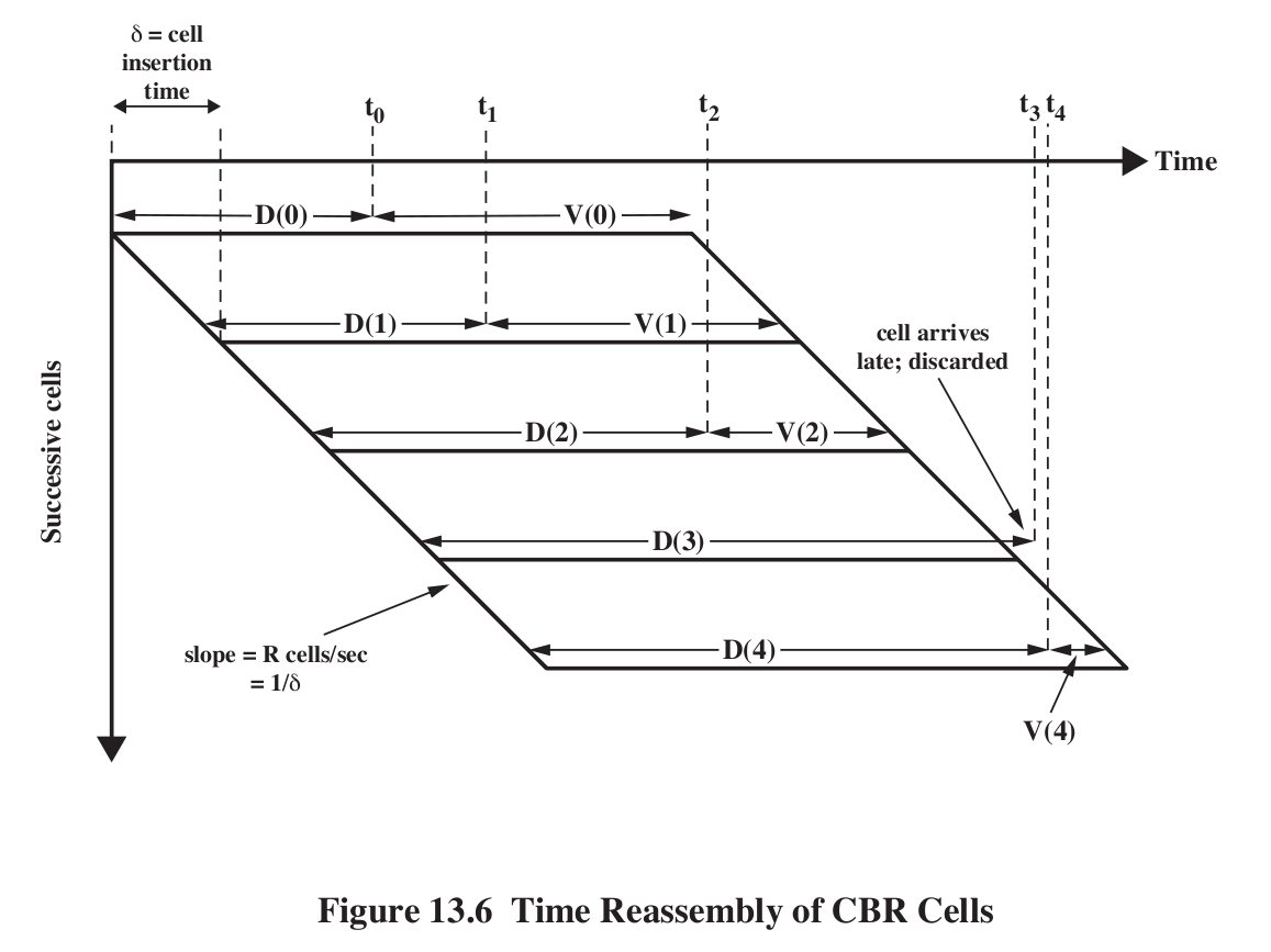
The first packet (packet 0) is sent at time T=0. Its propagation delay
is D(0). Upon arrival, the receiver holds it for an additional time
V(0), to accommodate possible fluctuations in future D(i). Packet
transmission time for the ith packet is k*i, where k is the packet
sending interval (eg 6 ms for 48-byte ATM cells). The ith packet arrives
at k*i + D(i). Let T be the time when we play back the first packet,
D(0)+V(0); this is the time between sending and playing. Then for each
i, D(i) +V(i) = T, so V(i) = T-D(i). Also, the ith packet needs to be
played back at T+k*i. A packet is late (and thus unuseable) if D(i)>T.
V(0) is thus the value chosen for the initial receiver-side "playback
buffering time". If the receiver chooses too small a value, a larger
percentage of subsequent packets/cells may arrive too late. If V(0) is
too large, then too much delay has been introduced. Once V(0) is
chosen, all the subseequent V(i) are fixed, although there are algorithms to adapt T itself up or down as necessary.
V(0) (or perhaps, more precisely, the mean value of all the V(i)) is also known as the depacketization delay.
Suppose we know (from past experience with the network) the mean delay meanD, and also the standard deviation in D, which we'll call sd (more or less the same as CDV, though that might be mean deviation rather than standard
deviation). Assuming that we believe the delay times are normally
distributed, statistically, we can wait three standard deviations and
be sure that the packet will have arrived 99.99% of the time; if this
is good enough, we can choose V(0) = meanD + 3*sd - D(0), which we
might just simplify to 3*sd. If we want to use CDV, statistical
theory suggests that for the same 99.99% confidence we might want to
use 4*CDV. In general, we're likely to use something like V(0) =
k1 + k2*CDV.
Sometimes the D(i) are not
normally distributed. This can occur if switch queues are
intermittently full. However, that is more common in IP networks than
voice-oriented networks. On a well-behaved network, queuing theory puts
a reasonable value of well under 1 ms for this delay (Walrand
calculates 0.07 ms).
Note that the receiver has no value for D(0), though it might have a pretty good idea about meanD.
Note that the whole process depends on a good initial value V(0); this determines the length of the playback buffer.
V(n) is negative if cell n simply did not arrive in time.
For IP connections, the variation in arrival time can be hundreds of milliseconds.
Computed arrival time; packets arriving late are discarded.
Note that
increased jitter
=> increased estimate for V(0)
=> increased overall delay!!!
Congestion issues generally
Congestion occurs at entry queues to links. Congestion is usually defined to be (taildrop) losses, but the term may also refer to queue buildup.
Congestion may simply result in increased delay at constant throughput
(best case). But it also may result in plummeting throughput; as
offered_load -> 100%, perhaps delay -> infinity!
retransmission saturation: suppose A sends to D, B to C, C to B, and D
to A, all sending clockwise (ABD, BDC, DCA, CAB). Suppose each sender
offers rate r<1, where 1 is the maximum rate.
A-----B
| |
| |
C-----D
Now suppose that at each router the loss-ratio is α<=1.
Traffic from A to B (thus, the load offered to router B) consists of:
- load r, offered by host A
- load (1-α)r, initially offered by C, and lost at A.
Further, let us assume that if the offered load exceeds 1, then the router reduces the load proportionally.
The total load is r + (1-α)r. For r≥0.5, we can solve for α: α =
(2r-1)/r. When r=1/2, α=0 (no losses). As r⟶1, however, we see α⟶1,
that is, 100% loss rate. [ref: Kurose & Ross, Computer Networking
5e, §3.6, Scenario 3]
ATM
GCRA [generalized cell rate algorithm], CAC [connection admission control]
(GCRA defined later)
CBR = rt-VBR with very low value for BT (token bucket depth)
rt-VBR: still specify maxCTD; typically BT is lower than for nrt-VBR
nrt-VBR: simulates a lightly loaded network; there may be bursts from other users
Circuit setup involves negotiation of parameters
Things switches can control:
- Admission Control (yes/no to connection)
- Negotiating lower values (eg lower SCR or BT) to a connection
-
Path selection, internally
-
Allocation of bandwidth and buffers to individual circuits/paths
-
Reservations of bandwidth on particular links
-
Selective dropping of (marked) low-priority cells
-
ABR only: asks senders to slow down
-
Policing
Congestion control mechanisms generally: ch 13.2, fig 9e:13.5
-
backpressure (good for x.25): a router sends slowdown indication to previous hop router
-
choke packets (ICMP source quench): send slowdown to the source
-
Implicit signaling
-
coarse packet loss
-
fast-retransmit: detect loss of packet N due to arrival of N+1, N+2, and N+3 (sort of)
-
monitoring of increasing RTT
-
Explicit signaling - various forms
-
DECbit style (or Explicit Congestion Notification)
-
Frame Relay: FECN, BECN bits (latter is more common)
credit-based: aka window-based; eg TCP
rate-based: we adjust rate rather than window size
Note that making a bandwidth reservation may still entail considerable per-packet delay!
Some issues:
-
Fairness
-
QoS
-
Reservations
-
multiple queues, "fair queuing"
-
fair queuing and window size / queue usage
Any congestion-management scheme MUST encourage "good" behavior: we
need to avoid encouraging the user response of sending everything
twice, or sending everything faster.
ATM congestion issues:
-
RT traffic not amenable to flow control
-
feedback is hard whenever propagation delays are significant
- bandwidth requirements vary over several orders of magnitude
-
different traffic patterns and application loss tolerance levels
-
latency/speed issues
Latency v Speed:
transmission time of a cell at 150 Mbps is
about 3 microsec. RTT propagation delay cross-country is about 50,000
microsec! We can have ~16,000 cells out the door when we get word we're
going too fast.
Note that there is no ATM sliding-windows mechanism!
CLP bit: negotiated traffic contract can:
- Cover both CLP=0 and CLP=1 cells; ie CLP doesn't matter
- Allow sender to set CLP; contract covers CLP=0 cells only; carrier may drop CLP=1 cells
- Allow network to set CLP; CLP set to 1 only for nonconforming cells
Section 13.5 (towards the end)
Suppose a user has one contract for CLP=0 traffic and another for CLP-0-or-1 traffic. Here is a plausible strategy:
cell
|
compliance
|
action
|
CLP = 0
|
compliant for CLP = 0
|
transmit
|
CLP = 0
|
compliant for CLP-0-or-1
|
set CLP=1, transmit
|
CLP = 0
|
noncompliant for CLP-0-or-1
|
drop
|
CLP = 1
|
compilant for CLP-0-or-1
|
transmit
|
CLP = 1
|
noncompliant for CLP-0-or-1
|
drop
|
A big part of GFR is to make sure that all the cells of one larger IP
frame have the same CLP mark, on entry. A subscriber is assigned a
guaranteed rate, and cells that meet this rate are assigned a CLP of 0.
Cells of additional frames are assigned CLP = 1.
QoS agreements are usually for an entire Virtual Path, not per-Virtual-Channel.
That is, the individual channels all get one lump QoS, and the endpoints are responsible for fairness among the VCCs
Traffic policing v shaping (essentially provider-based v sender-based)
Token bucket (fig 89e:13.11) is usually construed as a shaping algorithm:
note smoothing effect on big bursts, but ability to pass smaller bursts
intact.
Algorithm: tokens accumulate at a rate r, into a bucket with maximum
capacity D (=bucket depth). This is done by the token generator. The
sender needs to take a token out of the bucket (ie decrement the token
count) each time it sends a packet.
Token bucket with bucket size s=1, initially full, rate r=1/5
Conformant:
0 5 10 15 20 ...
0 6 11 16 21
NOT: 0 6 10 ...
NOT: 0 4 ...
Token bucket with size s=1.2, initially full, rate r=1/5
This is now conformant:
0 6 10 16 20 ...
GCRA
GCRA - Generalized Cell Rate Algorithm (called UPC algorithm in Stallings, 13.6)
GCRA is a form of leaky / token bucket
(these
are two ways of describing the same fundamental process. leaky bucket:
cells add to bucket; can't overflow it; transmission fluid leaks out;
token bucket: cells subtract from bucket; volume can't go negative,
transmission fluid comes in)
GCRA(T,𝝉): T = average time between packets, 𝝉 = tau = variation
We define "theoretical arrival time", or tat, for each cell, based on the arrival time of the previous cell.
Cells can always arrive later, but not earlier.
Arriving late doesn't buy the sender any "credit", though (in this sense, the bucket is "full")
Initially tat = current clock value, eg tat=0.
Suppose the current cell is expected at time tat, and the expected cell spacing is T.
Let t = actual arrival time
Case 1: t < tat - 𝝉 (the cell arrived too EARLY)
- mark cell as NONCONFORMING
- do not change tat (applies to next cell)
Case 2: t >= tat - 𝝉
- cell is CONFORMING
-
newtat = max(t,tat) + T
draw picture of t<tat-𝝉, tat-𝝉<= t < tat and tat < t. The last case is "late"
Examples: GRCA(10,3) for the following inputs
0, 10, 20, 30
0, 7, 20, 30
0, 13, 20, 30
0, 14, 20, 30
1, 6, 8, 19, 27
CGRA(3,12):
arrivals: 0,0,0,0, 0, 3, 9,10,15
tats: 0,3,6,9,12,15,18,21,24
What is "fastest" GRCA(3,16) sequence?
peak queue length is approx 𝝉/T
better: 𝝉/(T-1) + 1
Token bucket: accumulate "fluid" at rate of 1 unit per time unit.
Bucket capacity: T+𝝉; need T units to go (or (T+𝝉)/T, need 1 unit)
A packet arriving when bucket contents >= T is conforming.
Conformant response: decrement bucket contents by T.
Nonconformant response: do nothing (but maybe mark packets)
Token bucket formulation of GCRA:
- bucket size T+𝝉
- bucket must contain T units at cell arrival time
- No: nonconformant
- Yes: take out T units
CLP bit and conformant/nonconformant
CBR traffic
1. Specify PCR and CDVT. We will assume PCR is represented as cells per cell transmission time.
2. meet GCRA(1/PCR, CDVT)
What does this mean?
6 ms sending rate, 3 ms CDVT
cells can be delayed by at most CDVT!
VBR traffic (both realtime and nrt)
GCRA(1/PCR, CDVT) and GCRA(1/SCR, BT+CDVT)
Note CDVT can be zero!
What does big 𝝉 do?
Example: PCR = 1 cell/microsec
SCR = 0.2 cell/microsec
CDVT = 2 microsec
BT = 1000 cells at 0.2 cell/microsec = 200 microsec
GCRA(1,2): delay cells by at most 2 microsec
GCRA(5,200): would have allowed delay of 200 microsec, but disallowed by first.
Allow 0 1 2 3 ... 999 5000
rt v nrt? Generally the latter has larger BT values (as well as not
being allowed to specify maxCTD, and generally having a much larger
value for meanCTD).
For both CBR and VBR traffic, the sender may negotiate separate values for CLP 0 and CLP 0+1 traffic.
traffic shaping:
VBR traffic can be SHAPED, say by emitting cells at intervals of time T.
This works for nrt-VBR, but will break CTD bound for rt-VBR
Example:
CGRA(3,12):
arrivals: 0,0,0,0, 0, 3, 9,10,15
tats: 0,3,6,9,12,15,18,21,24
GCRA(1,2) & GCRA(5,200):
These are traffic descriptions; the network only makes loss/delay promises
GCRA(1,2): At PCR 1/1, cells can be early by at most 2
GCRA(5,200): At SCR 1/5, cells can be early by 200.
But the 200 cells cannot arrive faster than PCR, by more than 2
ABR: available bit rate
UBR: unspecified bit rate
GFR: Guaranteed Frame Rate
For ABR, the network offers the PCR, subject to being >= the MCR.
For UBR, the user specifies the PCR and the CDVT.