In this file we present several examples of programs to test the behavior of the cache, and then an example of how one can write programs to take advantage of how the cache works.
The basic rule is that memory is fetched by the cache line (or cache block). On Intel processors a cache line contains 64 bytes. Fetches from memory itself are quite slow, but fetches from the cache are reasonably fast. The CPU cannot tell, when it is executing an instruction that accesses memory, whether the data is in the cache or not, though it will find out by how fast the instruction executes.
On a linux system one can find the cache sizes with the command lscpu. On my laptop this yields
L1d
cache:
32K (data cache)
L1i cache:
32K (instruction lache)
L2
cache:
256K
L3
cache:
3072K
In this program we create a square matrix, and access it by row and then by column. Entries in the matrix are integers, and it is linear in memory. We access a given component via the rule
A[row,col] = A[row*WIDTH + col]
This means that, for a fixed row, the column values are consecutive in memory.
We create the matrix on the heap with malloc(). We then access the elements in row-major order (first all the columns of row 0, then all the columns of row 1, etc) and then in column-major order. Row-major order amounts to linear access of the underlying memory allocation; column-major order skips around.
void
roworder( int * A) {
int row, col;
for (row=0; row<HEIGHT; row++) {
for (col=0; col< WIDTH;
col++) {
A[row*WIDTH + col] = 0;
}
}
}
Row-major order is faster. If all memory accesses really were equal, it would not be. For WIDTH=10000 and height=8000 (320 MB), the difference is a factor of 5-6.
But as we make the ratio smaller, the ratio falls. For a 16 MB matrix (2000 x 2000), it is ~3.5; a 4 MB matrix (1000 x 1000) is similar.
But for 500x500, the ratio falls to 1.1. That's because this array is 1 MB, and easily fits entirely within the cache. There is an initial pass over the entire array, which we do not include in the timings, that has the effect of loading the entire array into the cache.
At 600x600, which is 1.44 MB, or about half the cache, the time ratio rises to around 2.0. For 700x700 (~2 MB), the ratio varies from 2.0 to 4.0.
In this program we linearly access an array of memory of size 2N bytes (2N-2 integers). We count the total time.

The huge increase starting at N=22 (4 MB) indicates that, above this point, the entire array cannot be kept in the L3 cache. As we cycle around, new memory loads cause the cache to lose anything it had previously stored, by the time we get back to accessing the earlier part of the cache again.
We an also see a modest increase around N>15 (N=15 represents the size of the L1 data cache, 32 KB). The L2 cache size is N=18 (256 KB); we see another time increase at N=19. It is likely that at N=18 the entire array can be kept in the L2 cache, as the program code can stay in the L1 instruction cache.
This program is based on one at igoro.com/archive/gallery-of-processor-cache-effects, by Igor Ostrovsky. Though the bulk of that article seems to be about 2010-era CPUs. And it also uses examples in C#.
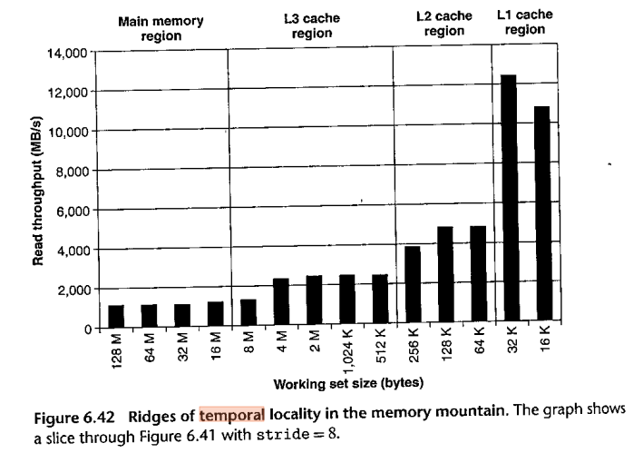
Here is the BOH3 version of this diagram, Fig 6.42. Note that it is reversed left to right, and also vertically as it measures throughput rather than delay. Still, the four "steps" (L1, L2, L3 and main memory) are more clearly defined than with my diagram.
But notice the dips in throughput at the left edges of the L3 and L2 regions.
In loop 1, we access every element of a large array (64 million integers). In loop 2, we access one element from each cache block, that is, one array out of every 16.
If all memory accesses were equal, the first loop should take 16 times longer. In fact, the ratio is around 223/56, or 4.0. To put it another way, accessing the first element of each cache line is about 25% the time needed to access the entire cache line.
In the Ostrovsky page, this is called "update every Kth int". For K=16, his experience was that the access times were nearly equal. That would make sense if the entire cache line had to be loaded before any data could be accessed.
I added 1 to each array entry; Ostrovsky multiplied by 3. This did not make any difference.
In this example we try to get a sense of the extent of cache prefetch: if we access one cache line, will the next one be prefetched? We create a long array of size 1,000,003 x 64 bytes, or 1000003 cache lines. We access the lines at intervals, going from line i to line i+skip:
skip=1: 0,1,2,3,4,5,6,...
skip=2: 0,2,4,6,8,...
skip=3: 0,3,6,9,12,...
The skip sequences all eventually hit every cache line; it helps, for this purpose, that 1000003 is a prime number. When a skip sequence gets above 1000003, we wrap around modulo 1000003. Here is a graph showing the total time for skip from 1 to 100:

At skip =15, there is a sharp peak (it is not clear why, though 16 x 64 is about 1KB). After that, the time levels off. But in the range from 1 to 14, the time increases linearly with the skip value, suggesting that prefetching is a real effect. And also that the prefetch algorithm cannot handle fetches 16 lines ahead. No idea what the spike is at skip=95.
We'll just take Ostrovsky's example at igoro.com/archive/gallery-of-processor-cache-effects. It is based on a loop to update every Kth byte of a large array. Slower times result when the total number of values accessed exceeds the cache capacity. This accounts for the upper-left blue triangle.
But the thing we want to look at is the presence of the blue vertical lines. It turns out that caches cannot put a given chunk of memory anywhere. Some caches -- direct-mapped caches -- store the memory chunk starting at address 64*N at cache line N modulo (cache size). If the cache size is 1 MB, then memory blocks 0 -- 63 and 220 -- 220+63 get mapped to exactly the same cache line, and so accessing one will displace the other. Another way to put this is that any memory address A maps to the cache address (A mod 220); that is, the cache address is always just the low-order 20 bits of the original memory address.
Another cache architecture is N-way associative. This allows any memory block to be stored at up N different cache locations. N=16 is typical; in a 16-way cache if we access 17 blocks that each have the same set of cache locations, then the last access will have to overwrite one of the earlier accesses. Ostrowsky's cache is 16-way associative.
A final, and more expensive, cache architecture is fully associative.
If we are updating every 512th value in an 8 MB array (221 integers), that is 4096 values. Those should easily fit in the cache. However, many of those 4096 values are restricted, by the 16-way-associativity hardware, to being mapped to the same locations. Therefore, there is lots of cache overwriting and the attendant need to re-load the values.
Matrix multiplication involves accessing the second matrix by column. To find the matrix product A×B of two N×N matrices at row=r, col=c, we take the rth row of the first matrix A and the cth column of the second matrix B, form the sum of the product of each pair of corresponding entries. This means traversing the rth row of the first matrix linearly, which is well-behaved in terms of the cache, but then traversing the column of the second matrix, which is not.
One relatively simple way to handle this is first to transpose the second matrix, B, so that the columns of B are the rows of BT. Now, instead of traversing a column of B we can traverse a row of BT. Row traversal is, as always, cache-friendly. Creating BT is slow, but is only one traversal of the entire matrix; calculating the product is equivalent to N traversals of the entire matrix.
For 2000×2000 matrices, the time without transpose is ~21 seconds. With, it falls to under 4.0 seconds. This 5.2 factor is comparable to that in the rows_and_columns example above.
There are other algorithms for fast, cache-friendly matrix multiplication, and for other matrix operations.
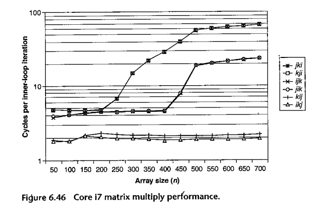
BOH3 has a rather different approach to the matrix-multiplication problem: rearrange the order of the three loops. Here is their code:
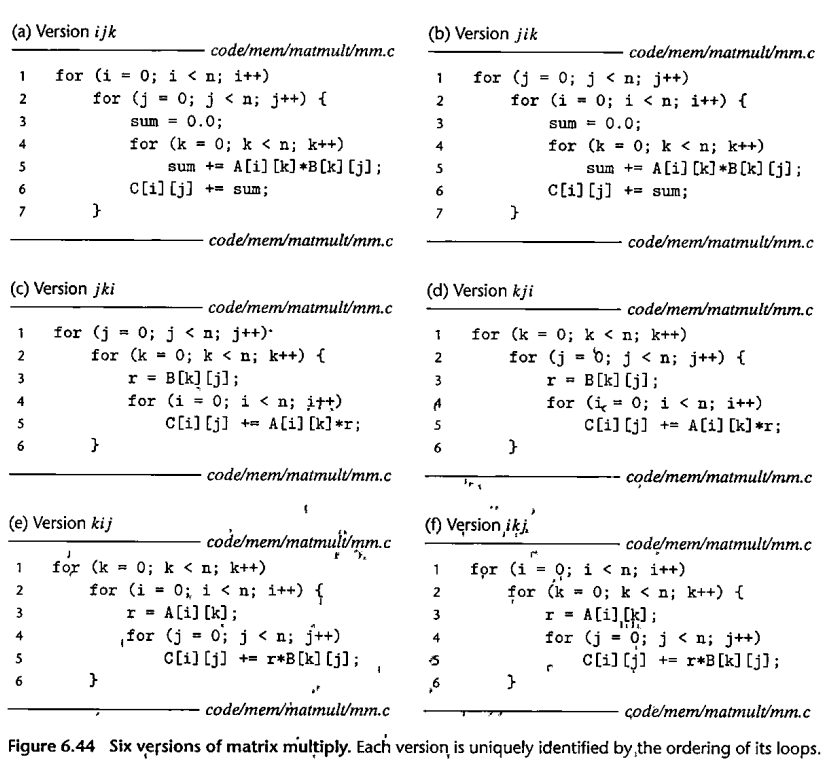
And here are their results:
Why does the ikj loop work so much faster? See row_i_col_multiply() in matrix2.c